Tous droits réservés pour tous pays. All rights reserved.
| Serveur © IRCAM - CENTRE POMPIDOU 1996-2005. Tous droits réservés pour tous pays. All rights reserved. |
Rapport Ircam 15/78, 1978
Copyright © Ircam - Centre Georges-Pompidou 1978
Abstract
The model is intended to simulate the stereophonic localization "response" and other important characteristics of the reproduced sound. It accepts the following parameters of the sound pick-up and reproduction svstems : the polar pattern and position of the microphones used (up to 4), the distance of the sound sources and their spectrum, the law-out of the loudspeakers and the psychoacoustics of sound localization. Traditional stereophonic systems are analysed and their performances compared.
Apart from pseudo-mono sound-pickup practices, for example the use of panoramic devices for mixing a large quantity of monopohonic microphones into two channels, sound engineers in different recording studios are using -- more or less empirically -- correct stereophonic systems. Many such systems have names such as EMI's "stereosonic" or the continental "XY" and "MS" -- others are known under the name of the institution using them (ORTF-France) -- some are anonymous and some belong in the "artificial head" category.
The aim of this paper is to develop a mathematical model of such stereophonic svstems, i.e., a model which permits an analysis of the most interesting performances, as a function of the microphone-sound source positions in the recording space, the interaction between room acoustics and microphone system, the characteristics of the microphones used, the lay-out of the speakers in the reproduction room and, finally, the psychoscoustics of sound localization.
Using our model, we compute the following results :
All the computation work was done on a Digital Equipment Corp. PDP-10 computer using SAIL, an ALGOL-based language developed at the Stanford Artificial Intelligence Laboratories. As the programmes are almost trivial, they are not included in this paper, but we would be happy to send more information to anyone who asks.
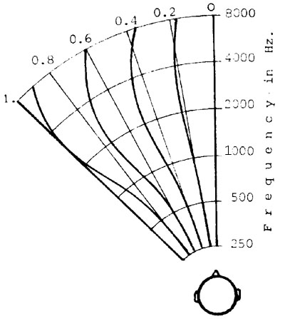
The interaural intensity difference (IID) as a function of the azimuth of a real sound source is computed by the equation :
{1}
where f is the frequency of the signal in KHz and IID is expressed as the ratio of sound pressures at the two ears. This equation represents an approximation of the experimental results of 9 authors [1]. In figure 1, this equation is represented by the dashed curves, while the average of the experimental results is represented by the solid curves.
Figure 1
IID's determined by the azimuth of the sound source
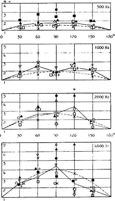
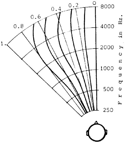
It must now be emphasised that the azimuth of a virtual sound source, as determined by the IID's, is a function quite different from that represented by equation III. Indeed, as some authors, for example Feddersen et al. [2] showed, the necessary IID for creating a certain angular localization is (a) frequency dependent and (b) larger than the "natural" IDD created by some real sound source disposed at the same angle. This assertion can be better understood from the figure 2, where the solid dark lines represent the experimental results of Feddersen, while the dashed curves represent our approximated equation :
{2}
The solid light curves in figure 2 represent the computed values of IID by the equation {1}.
Figure 2
The interaural time difference (ITD) as a function of the azimuth of the real sound source can be expressed as :
{3}
where h is the average distance between the two ears (~0.21m.), c is the speed of the sound in air (~ 0.34 m./msec.), and ITD is expressed in milliseconds.
While using the equation {3} we accept some minor errors (we ignore the frequency dependence caused by the contour of the head for example) in order to simplify the deductions which follow.
It is assumed that the perceived localization angle represents the algebraic sum of the localization angles determined by (a) interaural intensity differences and (b) interaural time differences [ 1; 2; 3; ].
The equation of IID (interaural intensity differences) determined by the stereophonic signals is [4] :
{4}
where k is the voltage ratio of the two stereophonic signals, m is the IID determined by the azimuth of one of the symmetrically disposed loudspeakers in the listening room.
To obtain the virtual localization angle determined by the IID's, we first calculate m by introducing the desired azimuth of the loudspeakers into equation {1}, then use m in equation {4} to obtain the IID (stereophonic), which we then use in equation {2}.
The virtual localization angle determined by the interaural time differences is represented [4] by the equation :
where alpha (o) is the azimuth of the loudspeaker with respect to the listener,
T(o) is the ITD determined by alpha (o) ;
T(s) is the time-delay between the two stereo signals ;
k is the voltage ratio of the two stereo signals and
m is the IID determined by alpha (o).
The variables k and T(s) depend on the polar patterns of the microphones used, their position in the recording space,
the distance between the sound source and the "center" of the microphone array, and, finally, the azimuth of the real
sound source. This azimuth was expressed not in absolute angles, but by the ratio of the sound source azimuth to the
maximal pick-up angle of the system ; this way we tried to avoid confusion in the comparision of real sound
source and virtual localization angle as the latter depends on the loudspeaker lay-out and on listener position.
The deductions used for the computation of k and T(s) can be found in the Appendix 1.
Finally, the virtual localization angle represents the algebraic sum of the localization angles determined by IID and
ITD :
The mono compatibility of stereo programmes has lost the
importance it had at the beginning of the stereo "era" ; nevertheless, the amount of monaural equipment
(especially radio receivers) still in use remains significant.
In this category, the quality of the mono signal is very important and we computed, on the basis of phase differences
between the stereo signals, the frequency response of the sum mono signal for all frequencies used and positions of
the sound-source. This frequency response is related to a sum signal with NO phase differences and is expressed in
decibels (details in Appendix 2).
Another important characteristic of a stereophonic system is, we think, its response to the acoustics of the recording
space. It is well known that certain stereophonic pick-up systems enhance the reverberation of the recording space
while other microphone placements and characteristics reduce the reproduced reverberation. We tried to analyse this
"response" by computing the ratio of the sound energy occurring in the direct sound angle (i.e. within the limits where
the desired sound source was located) to the total sound energy, The results are very interesting for both stereo and
monophonic reduction. Important chances in the reverberation "response" as a function of the signal frequency can be
observed, as well as a different reverberation effect for the mono sum signal.
{5}
{6}
Compatibility and reaction to the room acoustics
Coincident Systems
The first stereophonic coincident sound pick-up system, anticipated in 1931 by Blumlein [5], is the "Stereosonic", which
uses two figures of eight microphones with their main axes directed at +45 and -45 degrees respectively. The sound
sources must be placed within this angle. The results of the computation are shown in fig. 3. The azimuths of the
virtual sources are quite correct for the low frequencies but become less accurate as the frequency increases.
As expected, no differences of phase or incompatibilities of the mono and stereo signals are observed. As for the
reverberation "response", it can be seen that the monophonic sum signal is "drier" than the stereophonic one.
The performance of the system known by the name "XY" (still often used especially in Germany) which uses a cardioid polar pattern with the main axes at +45 and -45 degrees, is shown in fig. 5. Characteristic in such a system is the "compression" of the virtual sound sources into a space delimited by about half the angle of the loudspeakers. In other words, we obtain a "mono-like" image concentrated in the central space between the loudspeakers. The fact that the reverberation "response" is about the same for stereo or mono does not compensate for the poor quality of this system, which is recommended only for solo or for small ensembles.
Some better results are obtained if the axes of the cardioids are at +60 and -60 degrees (fig. 6).
(In all the tables and drawings the azimuths of the real sound sources ( > / >o) are represented as the ratio of the actual azimuth to the maximal pick-up angle of the system (steps of 0.2 from 0 to 1) ; the same representation is used for the azimuth of the virtual source, the reference angle being the azimuth of the left loudspeaker ( < / < o), in our examples 30 degrees. Due to a weakness in our model, the ratio is sometimes greater than 1, and is denoted by brackets [ ] ; it should be treated as 1.)
Figure 3
Stereosonic Coincident System, 45 deg. pick-up angle
Frequency : 250.00 Hertz 				RAST = 0.25	RATMO = 0.41
> / > o 	< / < o		phase		mono

.00		-.00		.00		.0
.20		.17		.00		.0
.40		.36		.00		.0
.60		.55		.00		.0
.80		.76		.00		.0
 1.00		[1.01]		.00		.0

Frequency : 500.0 Hertz
> / > o		< / < o		phase		mono

.00		-.00		.00		.0
.20		.18		.00		.0
.40		.36		.00		.0
.60		.56		.00		.0
.80		.78		.00		.0
1.00		[1.04]		.00		.0

Frequency : 1000.0 Hertz
> / > o		< / < o		phase		mono

.00		-.00		.00		.0
.20		.19		.00		.0
.40		.39		.00		1.0
.60		.60		.00		.0
.80		.85		.00		.0
1.00		[ 1.16]		.00		.0

Frequency : 2000.0 Hertz
< / > o		< / < o		phase		mono

.00		-.00		.00		.0
.20		.21		.00		.0
.40		.43		.00		.0
.60		.65		.00		.0
.80		.99		.00		.0
1.00		[ 1.41]		.00		.0

Frequency : 4000.0 Hertz
> / >		< / < o		phase		mono

.00		-.00		.00		.0
.20		.19		.00		.0
.40		.40		.00		.0
.60		.65		.00		.0
.80		.98		.00		.0
1.00		[ 1.47]		.00		.0

Frequency : 8000.0 Hertz
> / >		< / < o		phase		mono

.00		-.00		.00		.0
.20		.15		.00		.0
.40		.32		.00		.0
.60		.53		.00		.0
.80		.84		.00		.0
1.00		[1.38]		.00		.0
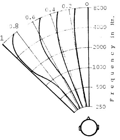
Figure 4
Cardioid Coincident Pair, 45 deg. pick-up angle
Frequency : 250.00 Hertz				RATST = 0.46	RATMO = 0.54
> / > o		< / < o		phase		mono

.00		-.00		.00		.0
.20		.07		.00		.0
.40		.14		.00		.0
.60		.22		.00		.0
.80		.29		.00		.0
1.00		.36		.00		.0

Frequency : 500.0 Hertz
> / > o		< / < o		phase		mono

.00		-.00		.00		.0
.20		.07		.00		.0
.40		.15		.00		.0
.60		.22		.00		.0
.80		.30		.00		.0
1.00		.37		.00		.0

Frequency : 1000.0 Hertz
> / > o		< / < o		phase		mono

.00		-.00		.00		.0
.20		.08		.00		.0
.40		.16		.00		.0
.60		.23		.00		.0
.80		.31		.00		.0
1.00		.40		.00		.0

Frequency : 2000.0 Hertz
> / > o		< / < o		phase		mono

.00		-.00		.00		.0
.20		.08		.00		.0
.40		.17		.00		.0
.60		.26		.00		.0
.80		.35		.00		.0
1.00		.44		.00		.0

Frequency : 4000.0 Hertz
> / > o		< / < o		phase		mono

.00		-.00		.00		.0
.20		.08		.00		.0
.40		.16		.00		.0
.60		.24		.00		.0
.80		.32		.00		.0
 1.00		.41		.00		.0

Frequency : 8000.0 Hertz
> / > o		< / < o		phase		mono

.00		-.00		.00		.0
.20		.06		.00		.0
.40		.12		.00		.0
.60		.19		.00		.0
.80		.25		.00		.0
1.00		.32		.00		.0
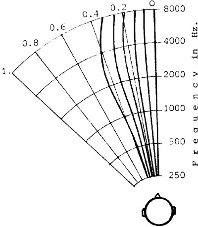
Figure 5
Cardioid Coincident Pair, 45 deg. pick-up angle
Frequency : 250.00 Hertz				RATST= 0.49	RATMO = 0.59
> / > o		< / < o		phase		mono

.00		.00		.00		.0
.20		.13		.00		.0
.40		.27		.00		.0
.60		.40		.00		.0
.80		.52		.00		.0
1.00		.64		.00		.0

Frequency : 500.0 Hertz
> / > o		< / < o		phase		mono

.00		.00		.00		.0
.20		.14		.00		.0
.40		.27		.00		.0
.60		.40		.00		.0
.80		.53		.00		.0
1.00		.64		.00		.0

Frequency 1000.0 Hertz
> / > o		< / < o		phase		mono

.00		.00		.00		.0
.20		.14		.00		.0
.40		.29		.00		.0
.60		.43		.00		.0
.80		.57		.00		.0
1.00		.71		.00		.0

Frequency 1000.0 Hertz
> / > o		< / < o		phase		mono

.00		.00		.00		.0
.20		.16		.00		.0
.40		.32		.00		.0
.60		.48		.00		.0
.80		.65		.00		.0
1.00		.81		.00		.0

Frequency : 4000.0 Hertz
> / > o		< / < o		phase		mono

.00		.00		.00		.0
.20		.14		.00		.0
.40		.29		.00		.0
.60		.45		.00		.0
.80		.61		.00		.0
1.00		.78		.00		.0

Frequency : 8000.0 Hertz
> / > o		< / < o		phase		mono

.00		.00		.00		.0
.20		.11		.00		.0
.40		.23		.00		.0
.60		.36		.00		.0
.80		.50		.00		.0
1.00		.65		.00		.0
The following example is a coincident system with two hypercardioid microphones directed at + 60 and - 60 degrees respectively. As fig. 7 illustrates, the localization is quite correct at the lower frequencies but exaggerated at the higher frequencies. The reverberation response is the same as for the 45 deg. XY system.
An artificial cross-talk frequency-dependent network can dramatically improve the localization response, as it can be seen in fig. 8 (details about the characteristics of the network will be soon available). The use of this network, the effect of which is similar to that of the "shuffler circuit" of Vanderlyn [6] can also improve the response of the "stereosonic" system (fig. 9).
Notice that the cross-talk network determines small changes in the reverberation "response" of both compensated systems ; as the changes are small, we mentioned only the upper and lower limits.
The first system we analyse is the so-called ORTF system, a pair of directional microphones with their main axes at +55 and -55 degrees, the distance between them being 17 cm. This system is widely used in French Broadcasting and special microphone constructions can be found in the catalogues of some manufacturers. The localization responses are acceptable, as can be seen in the figures 10 (cardioid pattern) and 11 (hypercardioid). Please notice that the phases are proportional to the sine of the azimuth of the sound source and are not frequency-dependent. The most important disadvantage is the very poor compatibilty. As an example, we calculated the 4000 Hz+ curve for azimuths of the sound source changing each 5 degrees and the frequency response of the mono signal for a source placed at an angle of 22 degrees (fig. 6).
Figure 6
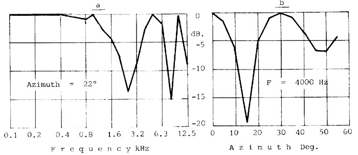
Figure 8
Hypercardioid Coincident Pair, compensated, pick-up angle 60 deg.
Frequency : 250.0 Hertz RATST = 0.46 - 0.49 RATMO = 0.66 - 0.74
> / > o		< / < o		phase		mono

.00		.00		.00		.0
.20		.20		.00		.0
.40		.40		.00		.0
.60		.59		.00		.0
.80		.79		.00		.0
1.00		.99		.00		.0

Frequency : 500.0 Hertz
> / > o		< / < o		phase		mono

.00		.00		.00		.0
.20		.20		.00		.0
.40		.39		.00		.0
.60		.59		.00		.0
.80		.79		.00		.0
1.00		.99		.00		.0

Frequency : 1000.0 Hertz
> / > o		< / < o		phase		mono

.00		.00		.00		.0
.20		.19		.00		.0
.40		.39		.00		.0
.60		.59		.00		.0
.80		.79		.00		.0
 1.00		[1.00]		.00		.0

Frequency : 2000.0 Hertz
> / > o		< / < o		phase		mono

.00		.00		.00		.0
.20		.19		.00		.0
.40		.39		.00		.0
.60		.59		.00		.0
.80		.80		.00		.0
1.00		[1.03]		.00		.0

Frequency : 4000.0 Hertz
> / > o		< / < o		phase		mono

.00		.00		.00		.0
.20		.18		.00		.0
.40		.37		.00		.0
.60		.57		.00		.0
.80		.80		.00		.0
1.00 		[1.06]		.00		.0

Frequency : 8000.0 Hertz
> / > o		< / < o		phase		mono

.00		.00		.00		.0
.20		.15		.00		.0
.40		.31		.00		.0
.60		.50		.00		.0
.80		.74		.00		.0
 1.00		[1.05]		.00		.0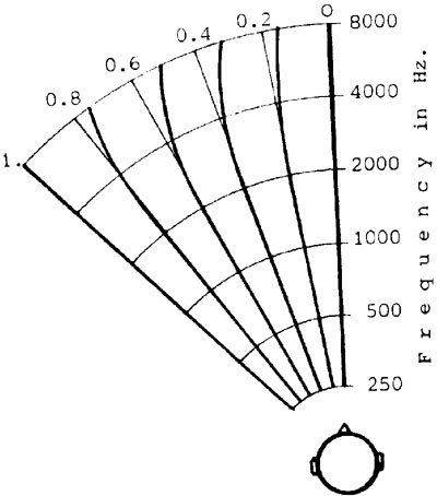
Figure 9
Stereosonic system compensated
Frequency : 250.00 Hertz RATST = 0.26 - 0.36 RATMO = 0.42 - 0.59
> / > o		< / < o		phase		mono

.00		-.00		.00		.0
.00		-.00		.00		.0
.20		.17		.00		.0
.40		.35		.00		.0
.60		.54		.00		.0
.80		.75		.00		.0
1.00		.99		.00		.0

Frequency : 500.0 Hertz
> / > o		< / < o		phase		mono

.00		-.00		.00		.0
.20		.17		.00		.0
.40		.35		.00		.0
.60		.54		.00		.0
.80		.75		.00		.0
1.00		.99		.00		.0

Frequency : 1000.0 Hertz
> / > o		< / < o		phase		mono

.00		-.00		.00		.0
.20		.17		.00		.0
.40		.34		.00		.0
.60		.53		.00		.0
.80		.74		.00		.0
 1.00		.99		.00		.0

Frequency : 2000.0 Hertz
> / > o		< / < o		phase		mono

.00 		-.00		.00		.0
.20		.16		.00		.0
.40		.34		.00		.0
.60		.53		.00		.0
.80		.74		.00		.0
1.00		[1.01]		.00		.0

Frequency : 4000.0 Hertz
> / > o		< / < o		phase		mono

.00		-.00		.00		.0
.20		.15		.00		.0
.40		.32		.00		.0
.60		.51		.00		.0
.80		.74		.00		.0
1.00		[1.03]		.00		.0

Frequency : 8000.0 Hertz
> / > o		< / < o		phase		mono

.00		-.00		.00		.0
.20		.13		.00		.0
.40		.27		.00		.0
.60		.45		.00		.0
.80		.68		.00		.0
1.00		[1.03]		.00		.0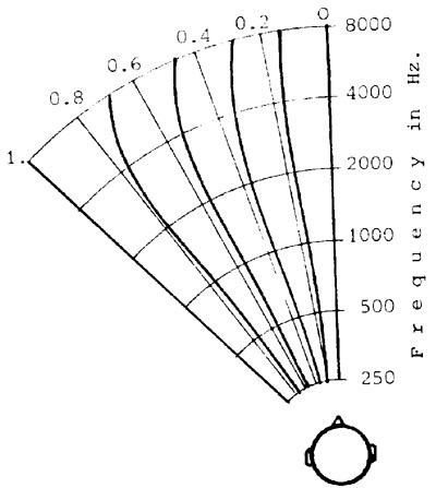
Figure 10
Ortf system, cardioid pattern
Frequency : 250.00 Hertz RATST = 0.49 RATMO = 0.41 - 0.60
> / > o		< / < o		phase		mono

.00 		-.01		.00 		.0
.20 		.13		-9.00		-.0
.40		.26		-17.00		-.1
.60		.39		-24.00		-.2
.80		.51		-31.00		-.3
1.00		.62		-37.00		-.3

Frequency : 500.0 Hertz
> / > o		< / < o		phase		mono

.00		-.01		.00		.0
.20		.14		-17.00		-.1
.40		.29		-34.00		-.4
.60		.43		-49.00		-.7
.80		.56		-62.00		-1.1
1.00		.67		-74.00		-1.4

Frequency : 1000.0 Hertz
> / > o		< / < o		phase		mono

.00		-.01		.00		.0
.20		.18		-34.00		-.4
.40		.35		-67.00		-1.5
.60		.52		-98.00		-3.2
.80		.66		-125.00		-4.7
1.00		.79		-147.00		-5.1

Frequency : 2000.0 Hertz
> / > o		< / < o		phase		mono

.00		-.01		.00		.0
.20		.22		-69.00		-1.6
.40		.44		-135.00		-7.5
.60		.64		164.00		-9.8
.80		.82		110.00		-3.6
1.00		.97		65.00		-1.1

Frequency : 4000.0 Hertz
> / > o		< / < o		phase		mono

.00		-4,01		.00		.0
.20		.25		-137.00		-8.5
.40		.50		90.00		-2.9
.60		.72		-32.00		-.3
.80		.91		-140.00		-5.9
1.00		[1.01]		130.00		-4.2

Frequency : 8000.0 Hertz
> / > o		< / < o		phase		mono

.00		-.01		.00		.0
.20		.27		85.00		-2.6
.40		.54		-179.00		-14.3
.60		.77		-64.00		-1.3
.80		.96		80.00		-1.9
1.00		[1.10]		-99.00		-2.5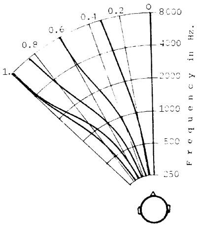
Figure 11
Ortf system, hypercardioid pattern
Frequency : 250.00 Hertz RATST = 0.47 RATMO = 0.45 - 0.70
> / > o		< / < o		phase		mono

.00		-.01		.00		.0
.20		.17		-9.00		-.0
.40		.36		-17.00		-.l
.60		.54		-24.00		-.2
.80		.70		-31.00		-.2
1.00		.87		-37.00		-.2

Frequency : 500.0 Hertz
> / > o		< / < o		phase		mono

.00		-.01		.00		.0
.20		.19		-17.00		-.1
.40		.39		-34.00		-.3
.60		.58		-49.00		-.6
.80		.75		-62.00 		-.8
1.00		.91		-74.00		-.6

Frequency : 1000.0 Hertz
> / > o		< / < o		phase		mono

.00		-.02		.00		.0
.20		.23		-34.00		-.4
.40		.46		-67.00		-1.4
.60		.67		-98.00		-2.7
.80		.86		-125.00		-2.9
 1.00		[1.01]		-147.00		-1.8

Frequency : 2000.0 Hertz
> / > o		< / < o		phase		mono

.00		-.02		.00		.0
.20		.27		-69.00		-1.6
.40		.55		-135.00		-6.6
.60		.81		-125.00		-2.9
.80		[1.04]		110.00		-2.4
 1.00		[1.24]		65.00		-.5

Frequency : 4000.0 Hertz
> / > o		< / < o		phase		mono

.00		-.02		.00		.0
.20		.30		-137.00		-8.3
.40		.60		90.00		-2.7
.60		.87		-32.00		-.3
.80		[1.11]		-140.00		-3.5
 1.00		[1.31]		130.00		-1.5

Frequency : 8000.0 Hertz
> / > o		< / < o		phase		mono

.00		-.01		.00		.0
.20		.31		85.00		-2.6
-40		.60		-179.00		-10.9
.60		.88		-64.00		-1.1
.80		[1.09]		80.00		-1.3
1.00		[1.26]		-99.00		-1.0
Systems with widely separated microphones, preferred in american studios, feature localization characteristics which are mainly time-delay dependent. That means that the virtual sources tend to spread with the frequency and, because of the important time-delays involved, to concentrate near the loudspeakers. The compatibility is fairly bad and the reverberation "response" is quite inconsistent and frequency-dependent. As a first example, we computed the characteristics of a system with omnidirectional microphones (i.e. with mainly time-dependent localization). The distance between the microphones is 3 m., the distance between the sound-source and the axis of the system is 4 and 8 m. respectively and the pick-up angle is 60 degrees. The results are shown in fig.12.
The fig.13 shows a similar system, the only difference being the polar pattern of the microphones which is a cardioid, with forward directed axes. No significant changes are apparent, except the reverberation response (fig.14).
It was (and, alas, sometimes still is... ) a widely used practice to "plug the hole between the loudspeakers" which appears during distanced-mike recordings by inserting a central microphone, the signal of which is routed with equal levels an the left and right chanels. The effect can be seen in fig.15 (3 cardioids, distance 1.5 m., distance of the source 8 m.).
An almost similar system is used for compensating the poor stereophonic effect of the XY-60 system : two cardioid microphones are placed at the left and right of the coincident one, their levels being set at approx -6 dB. The result (fig. 16) is a confusing localization pattern, with virtual sources "jumping" suddenly from left to right or vice versa ; the only quality of this arrangement is the good compatibility.
The computer-aided model of stereophonic systems seems to be an interesting tool for the analysis of different sound pick-up arrangements, although some minor errors determined by the approximation of the human localization ability have to be taken into account. It must be also emphasised that the polar patterns of the available microphones are (with the exception of the figure 8) different from the idealised patterns we had to consider for our computations.
Nevertheless it seems obvious that coincident techniques are by far better and that the use of distanced microphones or of combined systems should be where possible, avoided.
We would greatly appreciate any comments and suggestions, not only concerning our conception and computation techniques, but also for developments in more complex systems, such as quadraphonics.
Figure 12
Distanced omnidirectionals (D = 3m.), source at 4m. (Ieft-) and 8m. (right columns).
Frequency : 250.00 Hertz
> / > o		< / < o		phase		mono		< / < o		phase		mono

.00		.00		.00		.0		.00		.00		.0
.20		.46		-155.00		-13.3		.48		-162.00		-16.3
.40		.86		55.00		-1.0		.89		42.00		-.6
.60		[1.17]		-86.00		-2.7		[1.21]		-101.00		-4.0
.80		[1.40]		149.00		-11.4		[1.43]		135.00		-8.3
1.00		[1.56]		45.00		-.7		[1.58]		35.00		-.4

Frequency : 500.0 Hertz
> / > o		< / < o		phase		mono		< / < o		phase		mono

.00		.00		.00		.0		.00		.00		.0
.20		.73		50.00		-.9		.77		35.00		-.4
.40		[1.28]		110.00		-4.8		[1.32]		83.00		-2.5
.60		[1.64]		-172.00		-22.7		[1.68]		157.00		-14.1
.80		[1.87]		-62.00		-1.3		[1.89]		-91.00		-3.1
1.00		[2.01]		91.00		-3.1		[2.03]		71.00		-1.8

Frequency : 1000.0 Hertz
> / > o		< / < o		phase		mono		< / < o		phase		mono

.00		.00		.00		.0		.00		.00		.0
.20		[1.09]		100		-3.9		[1.13]		70.00		-1.8
.40		[1.73]		-141.00 	-9.5		[1,76]		167,00		-18.7
.60		[2.05]		17,00		-.1		[2.08]		-46,00		-47
.80		[2.24]		-124.00		-6.6		[2.26]		178.00		-36.2
1.00		[2.35]		-179.00		-37.9		[2,35]		142.00		-9.6

Frequency : 2000.0 Hertz
 > / > o	< / < o		phase		mono		< / < o		phase		mono

.00		.00		.00		.0		.00		.00		.0
.20		[1.48]		-160,00		-15.0		[1.52]		141.00		-9.5
.40		[2.08]		78.00		-2.2		[2.12]		-27.00		-.2
.60		[2.35]		34.00		-.4		[2.37]		-91.00		-3.1
.80		[2.48]		112.00		-5.0		[2.49]		-4,00		-.0
1.00		[2.56]		3.00 		-.0		[2.57]		-77.00		-2.1

Frequency : 4000.0 Hertz
 > / > o	< / < o		phase		mono		< / < o		phase		mono

.00		.00		.00		.0		.00		.00		.0
.20		[1.81]		41.00		-.6		[1.85]		-78.00		-2.2
.40		[2.33]		157.00		-13,9		[2.36]		-53.00		-1.0
.60		[2.53]		68.00		-1.6		[2.55]		177.00		-33.0
.80		[2.63]		-137.00		-8.7		[2.64]		-7.00		-.0
1.00		[2.69]		6,00		-.0		[2.69]		-154.00		-13.0

Frequency : 8000.0 Hertz
> / > o		< / < o		phase		mono		< / < o		phase		mono

.00		.00		.00		.0		.00		.00		.0
.20		[2.05]		82.00		-2.4		[2.08]		-156		-13.8
.40		[2.48]		-47,00		-.7		[2.50]		-106.00		-4.4
.60		[2.64]		135.00		-8.4		[2.65]		-5.00		-.0
.80		[2.72]		86,00		-2.7		[2.73]		-14.00		-.1
 1.00		[2.76]		12,00		-.0		[2.77]		52.00		-.9
Figure 13
Distanced cardioids (D = 3m.), source at 4m. (Ieft-) and 8m. (right columns).
Frequency : 250.00 Hertz
> / > o		< / < o		phase		mono		< / < o		phase		mono

.00		.00		.00		.0		.00		.00		.0
.20		.46		-155.00		-13.3		.48		-162.00		-16.3
.40		.86		55.00		-1.0		.89		42.00		-.6
.60		[1.17]		-86.00		-2.7		[1.21]		-101.00		-4.0
.80		[1.40]		149.00		-11.4		[1.43]		135.00		-8.3
1.00		[1.56]		45.00		-.7		[1.58]		35.00		-.4

Frequency : 500.0 Hertz
> / > o		< / < o		phase		mono		< / < o		phase		mono

.00		.00		.00		.0		.00		.00		.0
.20		.73		50.00		-.9		.77		35.00		-.4
.40		[1.28]		110.00		-4.8		[1.32]		83.00		-2.5
.60		[1.64]		-172.00		-22.7		[1.68]		157.00		-14.1
.80		[1.87]		-62.00		-1.3		[1.89]		-91.00		-3.1
1.00		[2.01]		91.00		-3.1		[2.03]		71.00		-1.8

Frequency : 1000.0 Hertz
> / > o		< / < o		phase		mono		< / < o		phase		mono

.00		.00		.00		.0		.00		.00		.0
.20		[1.09]		100		-3.9		[1.13]		70.00		-1.8
.40		[1.73]		-141.00 	-9.5		[1,76]		167,00		-18.7
.60		[2.05]		17,00		-.1		[2.08]		-46,00		-47
.80		[2.24]		-124.00		-6.6		[2.26]		178.00		-36.2
1.00		[2.35]		-179.00		-37.9		[2,35]		142.00		-9.6

Frequency : 2000.0 Hertz
> / > o		< / < o		phase		mono		< / < o		phase		mono

.00		.00		.00		.0		.00		.00		.0
.20		[1.48]		-160,00		-15.0		[1.52]		141.00		-9.5
.40		[2.08]		78.00		-2.2		[2.12]		-27.00		-.2
.60		[2.35]		34.00		-.4		[2.37]		-91.00		-3.1
.80		[2.48]		112.00		-5.0		[2.49]		-4,00		-.0
 1.00		[2.56]		3.00 		-.0		[2.57]		-77.00		-2.1

Frequency : 4000.0 Hertz
> / > o		< / < o		phase		mono		< / < o		phase		mono

.00		.00		.00		.0		.00		.00		.0
.20		[1.81]		41.00		-.6		[1.85]		-78.00		-2.2
.40		[2.33]		157.00		-13,9		[2.36]		-53.00		-1,0
.60		[2.53]		68.00		-1.6		[2.55]		177.00		-33.0
.80		[2.63]		-137.00		-8.7		[2.64]		-7.00		-.0
1.00		[2.69]		6,00		-.0		[2.69]		-154.00		-13.0

Frequency : 8000.0 Hertz
> / > o		< / < o		phase		mono		< / < o		phase		mono

.00		.00		.00		.0		.00		.00		.0
.20		[2.05]		82.00		-2.4		[2.08]		-156		-13.8
.40		[2.48]		-47,00		-.7		[2.50]		-106.00		-4.4
.60		[2.64]		135.00		-8.4		[2.65]		-5.00		-.0
.80		[2.72]		86,00		-2.7		[2.73]		-14.00		-.1
1.00		[2.76]		12,00		-.0		[2.77]		52.00		-.9
Figure 14
Rerverberation "Response" of distanced systems (see fig.12 & 13)
OMNIDIRECTIONAL -- 4m.			CARDIOID -- 4m.

Frequency : 250.00 Hertz		Frequency: 250.00 Hertz
RATST =		RATMO =			RATST =		RATMO =
	.22		.15			.53		.38

Frequency : 500.00 Hertz		Frequency : 500.00 Hertz
RATST =		RATMO =			RATST =		RATMO =
 	.22		.21			.53		.50

Frequency : 1000.00 Hertz		Frequency : 1000.00 Hertz
RATST =		RATMO =			RATST =		RATMO =
 	.22		.24			.53		.58

Frequency : 2000.00 Hertz		Frequency : 2000+00 Hertz
RATST =		RATMO =			RATST =		RATMO =
	.22		.26			.53		.61

Frequency : 4000.00 Hertz		Frequency : 4000.00 Hertz
RATST =		RATMO =			RATST =		RATMO =
	.22		.24			.53		.52

Frequency : 8000.00 Hertz		Frequency : 8000.00 Hertz
RATST =		RATMO =			RATST =		RATMO =
	.22		.25			.53		.63

OMNIDIRECTIONAL -- 8m.			CARDIOID -- 8m.

Frequency : 250.00 Hertz		Frequency : 250.00 Hertz
RATST =		RATMO =			RATST =		RATMO =
 	.30		.23			.69		.55

Frequency : 500.00 Hertz		Frequency : 500.00 Hertz
RATST =		RATMO =			RATST =		RATMO =
	.30		.29			.69		.66

Frequency : 1000.00 Hertz		Frequency : 1000.00 Hertz
RATST =		RATMO =			RATST =		RATMO =
	.30		.31			.69		.70

Frequency : 2000.00 Hertz		Frequency : 2000.00 Hertz
RATST =		RATMO =			RATST =		RATMO =
	.30		.36			.69		.75

Frequency : 4000.00 Hertz		Frequency : 4000.00 Hertz
RATST =		RATMO =			RATST =		RATMO =
	.30		.28		.69		.70

Frequency : 8000.00 Hertz		Frequency : 8000-00 Hertz
RATST =		RATMO =			RATST =		RATMO =
	.30		.30			.69		.68
Figure 15
Combined 3 cardioids directed forwards
Frequency : 250.00 Hertz
> / > o		< / < o		phase		mono

.00		.00		.00		.0
.20		.54		.120		-5.5
.40		.79		59.00		-1.2
.60		.73		-139.00		-8.1		RATST =		RATMO =
.80		[1.09]		103.00		-4.1			.58		.46
1.00		[1.30]		27.00		-.2

Frequency : 500.0 Hertz
> / > o		< / < o		phase		mono

.00		.00		.00		.0
.20		.68		33.00		-.4
.40		.82		65.00		-1.4
.60		[1.47]		-173.00		-10.3		RATST =		RATMO =
.80		[1.45]		-118.00		-5.2			.61		.54
1.00		[1.76]		54.00		-1.0

Frequency : 1000.00 Hertz
> / > o		< / < o		phase		mono

.00		.00		.00		.0
.20		.43		95.00		-3.0
.40		[1.02]		-164.00		-8.5		RATST =		RATMO =
.60		[1.73]		-39.00		-.5			.69		.70
.80		[2.07]		-165.00		-9.2
1.00		[2.09]		114.00		-5.0

Frequency 2000.0 Hertz
> / > o		< / < o		phase		mono

.00		.00		.00		.0
.20		[1.42]		120.00		-4.4
.40		[1.85]		-21.00		- .1		RATST = 	RATMO =
.60		[2.08]		-130.00		-7.2			.72		.77
.80		[2.33]		-3.00		-.0
1.00		[2.32]		-76.00		-2.0

Frequency 4000.0 Hertz
> / > o		< / < o		phase		mono

.00		.00		.00		.0
.20		[1.54]		-54.00		-1.0		RATST =		RATMO =
.40		[2.19]		-66.00		-1.5			.76		.77
.60		[2.44]		-145.00		-9.0
.80		[2.51]		-6.0		-.0
1.00		[2.64]		171.00		-15.2

Frequency 8000.0 Hertz
> / > o		< / < o		phase		mono

.00		.00		.00		.0
.20		[1.84]		-120.00		-5.1		RATST =		RATMO =
.40		[2.18]		-94.00		-2.9			.70		.68
.60		[2.52]		-5.00		-.0
.80		[2.63]		-22.00		-.2
1.00		[2.65]		58.00		-1.1
Figure 16
Combined coincident (XY) and distanced cardioids
Frequency : 250.00 Hertz
> / > o		< / < o		phase		mono
								RAST =		RATMO =
.00		.00		.00		.0			.76		.85
.20		.86 		-178.00		-4.2
.40		.21		-37.00		-.4
.60		[1.02]		67.00		-1.6
.80		[1.43]		-46.00		-.7
1.00		[1.58]		-146.00		-9.2

Frequency : 500.0 Hertz
> / > o		< / < o		phase		mono
								RAST =		RATMO =
.00		.00		.00		.0			.56		.56
.20		.50		-38.00		-.5
.40		[1.32]		-132.00		-4.3
.60		.67		-105.00		-2.4
.80		[1.85]		-99.00		-3.2
1.00		[1.75]		20.00		-.1

Frequency : 1000.0 Hertz
> / > o		< / < o		phase		mono
								RAST =		RATMO =
.00		.00		.00		.0			.56		.64
.20		-.48		-141.00		-2.0
.40		[1.51]		73.00		-1.8
.60		[2.02]		54.00		-1.0
.80		[2.22]		119.00		-4.6
1.00		[2.34]		-49.00		-.8

Frequency : 2000.0 Hertz
> / > o		< / < o		phase		mono
								RAST =		RATMO =
.00		.00		.00		.0			.60		.66
.20		[1.44]		57.00		-1.1
.40		[1.25]		-84.00		-1.6
.60		[2.34]		112.00		-4.0
.80		[2.52]		-79.00		-2.0
1.00		[2.59]		-117.00		-5.3

Frequency : 4000.0 Hertz
> / > o		< / < o		phase		mono		RAST =		RATMO =
.00		.00		.00		.0			.59		.65
.20		[1.80]		156.00		-3.7
.40		[2.30]		82.00		-2.3
.60		[2.48]		-85.00		-2.6
.80		[2.69]		161.00		-8.3
100		[2.44]		-109.00		-2.9

Frequency : 8000.0 Hertz
> / > o		< / < o		phase		mono
								RAST =		RATMO =
.00		.00		.00		.0			.51		.53
.20		[1.91]		-3.00		-.0
.40		[2.46]		-163.00		-7.57
.60		[2.61]		-41.00		-.6
.80		[2.71]		-4.00		-.0
1.00		[2.78]		35.00		-.4
Figure 17
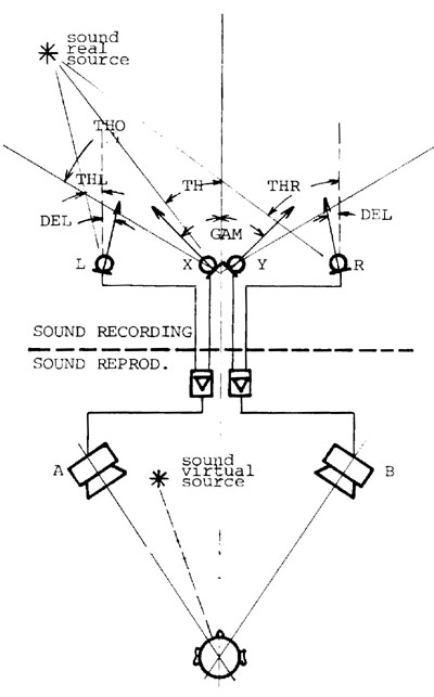
The equations of the microphones are :
For correct balance between the central and lateral microphones, Q + P and S + T must both equal. While considering the phase of the central microphones to be 0, the phases of the lateral microphones will be :
The sum left and right stereophonic signals will thus be :
The value of the time delay between the stereophonic signals A and B has to be computed on the basis of the individual timedelays and NOT on the basis of phase differences :
The derivation is based on the well-known Taylor expansion in which we neglect the second and higher power terms and get :
The computation of the phase between the signals A and B and of the monophonic sum signal is based on trivial trigonometric and other formula.
The computation of the reverberation "response" is based on the following assertions :
RATS = DIRST / REVST -- for stereophonic signals
RATMO = DIRMO / REVMO -- for monophonic signals
____________________________
Server © IRCAM-CGP, 1996-2008 - file updated on .
____________________________
Serveur © IRCAM-CGP, 1996-2008 - document mis à jour le .