Tous droits réservés pour tous pays. All rights reserved.
| Serveur © IRCAM - CENTRE POMPIDOU 1996-2005. Tous droits réservés pour tous pays. All rights reserved. |
ICMC 95, Banff (Canada), 1995
Copyright © Ircam - Centre Georges-Pompidou 1995
Physical models usually require the complete construction of a model for each new instrument. On the other hand our SSMs provide a methodology for modular construction of instruments [Tas94]. This construction is done automatically in our formal calculus environment. It allows to obtain different theoretical representations (state space equation, external or modal representation) and a synthesiser which simulates the instrument.
This paper focuses on the production of state space representation of hierarchical networks. Thus, we only briefly present the physical systems involved in wind instruments. We give some basics concerning the state space representation and we describe in detail the methodology that we used to combine modules together into networks of arbitrary complexity. In the third section, we apply this methodology to transmission lines, and in the last section we describe two software realizations of synthesiser builders.
In order to obtain a discrete model, the acoustic tube is spatially discretized in N elementary tubes of equal length and given section. This spatial discretisation is directly related to the sampling period which is the exact delay for a round trip in an elementary tube.
For a lossless tube the usual description of propagating waves in terms of superposition of ingoing and outgoing waves leads to the Kelly-Lochbaum structure. This structure is made of two delays and is parameterized by one reflection coefficient which represents the discontinuity between two elementary tubes. For state space description,s we prefer the lattice structure which is obtained by putting all the delays in the upper or in the lower branch of the lattice and by normalizing input and output waves [Mat90]. In that way we represent an acoustic tube by a quadripole system with an N-dimensional state space internal vector. As we normalize input and output waves of the acoustic tube in the lattice representation, we have to denormalize the inputs and the outputs of the whole system to obtain physical values.
When taking into account viscothermal losses, we prove that the acoustic
tube is still described by a generalization of the lattice filter.
Following the delay we add a filter which approximates the
frequency-dependent attenuation [Mat94]. The attenuation factor being proportional to  (where
  is the frequency), we use specific techniques to approximate it by a digital filter. We get the same structure for the state space equation than in the lossless case except for some scalars which are replaced by block matrices.
A wind instrument is an assembly of interconnected tubes. Connections of tubes are modeled by junction modules which implement Kirchoff's laws. At this time, we only consider two-port and three-port junctions. As in electrical circuit systems, networks have to be oriented. Consequently, we distinguish four three-port junctions.
 ,
,  and
and  are respectively the internal state vector, the input vector, and the
output vector.
are respectively the internal state vector, the input vector, and the
output vector.
Furthermore, a wide range of physical systems can be considered as linear dynamical systems. Then, the formal expression of such a model becomes (1.b) where the system is now represented by four matrices (A, B, C, D) respectively the matrix of dynamics, the control matrix, the observation matrix and the direct link matrix [Kai80]. These matrices are directly derived from the topology and the parameters of the system under study. Then building the model of an instrument is equivalent to establishing its four representative matrices. Once the representation is obtained, the system can be simulated by driving it with input vectors. If evolving in time, the system is described by time dependent matrices.
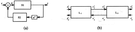
To build a network, we proceed by recursive combinations of two sub-systems. Considering two systems S1 and S2, they can be assembled (fig. 1) in a serial, parallel or feedback manner to create the system S. For these three combinations, the internal state space vector is
Figure 1: Serial (a), parallel (b) and feedback (c) connections of two modules.
= (1,2).
For the serial combination the output of S1 is connected to the
input of S2 and we have = 2 and = 1. For
the parallel combination, input and output are simply a concatenation :
= (1,2) and = (1,2). And for the
feedback combination, we have = 1 = 2 and = 1 - 2.
Notice that these combinations have been defined in order to construct networks in a very general way. They do not directly have a physical meaning. In particular, the connection of two acoustic tubes is not a simple serial connection but is done through the connection of two quadripoles which involves 4 serial, 2 parallel and 1 feedback connections (fig. 3).
For example, in order to identify an unknown parameter by using the Kalman extended filtering techniques, we classically add this parameter as an extra state space variable to the internal state vector. Consequently, we have to derive automatically a new state space equation corresponding to the enlarged state vector.
Establishing an external representation of physical systems is very
useful, for example, for performing real-time synthesis driven by physical
parameters. The synthesis becomes very efficient computationally
speaking. Such an external representation is obtained by
evaluating :
Modal representation of physical systems is well adapted to the context
of sound synthesis because of the structure of the sound output. Modal
synthesisers such as Modalys (previously known as Mosaic) need a
data base of modes adapted to the structure which is to be excited.
Modes can be obtained by establishing the state space equation for
the structure and by diagonalizing the matrix A of dynamics. This is
performed by formal or numerical calculus.

 is a transfer matrix and it reduces to a
scalar expression when input and output vectors are one-dimensional. In
this case
is a transfer matrix and it reduces to a
scalar expression when input and output vectors are one-dimensional. In
this case  is the transfer function corresponding to an ARMA
filter.
is the transfer function corresponding to an ARMA
filter.
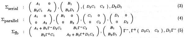
Global Representation of Linear Systems
In the linear case, a global representation ( A, B, C, D ) of a system network can be entirely deduced from the
representation ( Ai, Bi, Ci, Di ) of each of the components.
Serial, parallel and feedback connections are described in the
following equations where  + and are - respectively
set to (I - D1D2)-1, (I - D2D1)-1, with D1- = +D2.
+ and are - respectively
set to (I - D1D2)-1, (I - D2D1)-1, with D1- = +D2.
Modular Representation
The global approach for system representation is not efficient from a
computational standpoint: simulating a 50 cm tube at 44.1kHz
requires more than 6000 multiplication/additions per sample. To avoid
this problem we develop a modular approach which simulates
a whole system by propagating signal flows between modules.
This approach is similar to the one developed in
Music V, C-sound, Max, and waveguides.
We are interested in knowing in advance whether a network is computationally simulable or not. (By simulable we mean simply: ``capable of being simulated''.) Let S be a module network, S is simulable if its state equations (i.e.Figure 2: (a) Simulable feedback; (b) serial q-junction of two quadripoles.
and g) are explicit
expressions of the component module equations. By extension, we
will say that a module is simulable for a given type of
combination if any combination of the given type results in a
simulable network.
[n]
results from the following implicit equation [n] = g1([n] + g2([n])).
However, if the feedback loop is broken by at least one delay, as shown
in figure 2.a, we get an explicit expression for the
output ([n] = g1([n] + g2([n-1])))(see also [FC90]).
-, +), and outputs (+, -). These quadripoles may
be connected together with specific serial q-junctions (fig.
2.b) and parallel q-junctions12. These q-junctions are described as a hierarchical network of parallel, serial and feedback connections (fig. 3 and 4).
Figure 3: decomposition of a serial q-junction.
A serial q-junction between two quadripoles involves a feedback connection. It turns out that serial q-junctions of quadripoles can not be simulated in the general case, but can be simulated if each incriminated loop is broken by a delay.
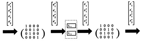
Figure 4: decomposition of a parallel q-junction.
We deduce some interesting properties: two quad-up connected in parallel is still a quad-up, a quad-up connected in serial with any quadripole is still a quad-up, two quad-up q-juncted together is simulable and is also a quad-up. One other interesting computational property of quad-up is that g (eq. 1.a) does not rely on e+ (resp. e- for quad-down). We deduce a simple algorithm for simulating the serial q-junction of two or more quad-ups.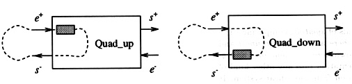
Figure 5: Two kinds of simulable quadripoles: the quad-up and the quad-down.
Notice that the most simple quadripole, i.e. the identity connection ( s+ = e+ and s- = e- ) is neither a quad-up nor a quad-down, and is therefore not simulable for serial q-junction purposes, which could become a drawback in the description of some transmission line networks.
If the network can be split in term of q-junctions, serial, parallel connections of oriented quad-ups and junctions without an oriented loop, then it is simulable, and is also a quad-up.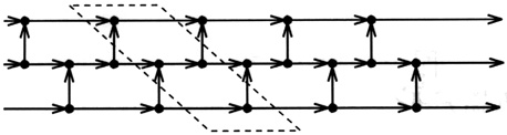
Figure 6: Network of transmission lines.
Fig. 7.a demonstrates how the network may be split into a regular pattern. Figure 7.b represents the pattern (a) as the parallel connection of different quad-ups. Thus this network is simulated by using simple basic elements (only J12 and J21 junctions). Of course this decomposition is not unique, and we could propose other combinations for this network.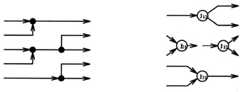
Figure 7: Network decomposition.
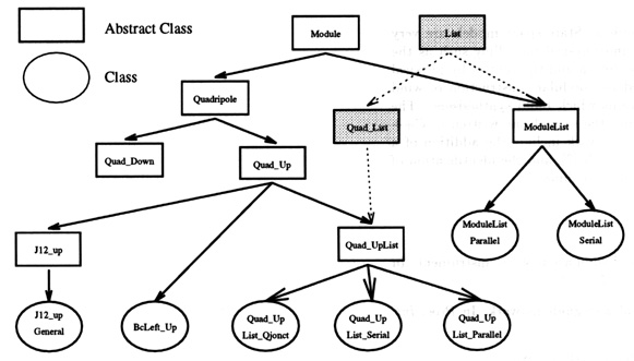
The Tube library is a library built around the statespace library which implements known linear models: cylindrical tubes with or without viscothermal losses, boundary conditions, junctions and T-junctions.
Usable objects are either Compound Modules[3], or any non-abstract class which implements a particular system. At this point we use parallel and serial connections, and q-junctions. We also implement classes which represent boundary conditions, tube models with or without viscothermal losses [Mat95], waveguide junctions [Tas94], non-linear reed models [Rod94]. This list may be completed by the implementation of other physical models.
Each non-abstract Module is described by an algorithm which computes an output from the inputs and its internal state. Some internal parameters (such as the reflection coefficient for a boundary condition) can be updated at run-time by a specific method. Others cannot (such as the length of a tube which cannot change dynamically).
We provide users with interactive interface with links, modules and
vectors for designing and simulating systems and for controlling the
synthesis with time-varying parameters.
Figure 8: Inheritance tree for the Module class.
Conclusion
We have considered here sound synthesis using state space models. State
space models are very promising since they keep the positive aspects of both
signal and physical modelling such as the ability for automatic extraction of
parameters, the internal description and the control by
physical parameters. We described the methodology that we
developed for modular construction of wind instruments and software
realizations of formal calculus programs which build synthesisers. The
first one written in Maple is devoted to theoretical purposes and the
second one written in C++ is devoted to sound synthesis. Future
development plans for this work include the addition of a fractional
delay module in order to simulate tubes of arbitrary length
[Val94], and the identification of unknown physical
parameters through the use of Kalman filtering techniques.
____________________________ ____________________________References
Notes
1 A Parralel q-junction is defined as - = (-1, -2), + = (+1, +2), + = (+1, +2), and - = (-1, -2).
2 There is no sense in defining a q-feedback for quadripoles.
Server © IRCAM-CGP, 1996-2008 - file updated on .
Serveur © IRCAM-CGP, 1996-2008 - document mis à jour le .