
Tous droits réservés pour tous pays. All rights reserved.
| Serveur © IRCAM - CENTRE POMPIDOU 1996-2005. Tous droits réservés pour tous pays. All rights reserved. |
Psychological Research, 58, 177-192 (1995)
Copyright © Psychological Research 1995
Submitted: 3 September 1994. Revised: 17 May 1995
Multidimensional scaling (MDS) has been a fruitful tool to study the perceptual relationships among stimuli and to analyze the underlying attributes used by subjects when making (dis)similarity judgments on pairs of stimuli ([Kruskal, 1964a,1964b]; [Shepard, 1962a,1962b]). The object of MDS is to reveal relationships among a set of stimuli by representing them in a low-dimensional (usually Euclidean) space so that the distances among the stimuli reflect their relative dissimilarities. To achieve this representation, dissimilarity data arising from N sources, usually subjects, each relating J objects pairwise, is modeled by one of a family of MDS procedures to fit distances in some type of space, generally Euclidean or extended Euclidean of low dimensionality R. The different dimensions are then interpreted as psychologically meaningful attributes underlying the judgments. An important distinction among different MDS techniques (that we will discuss below) is the kind of spatial model used to represent the distances between pairs of stimuli.
Multidimensional scaling of (dis)similarity judgments has been the tool of predilection for exploring the perceptual representation of timbre (e.g. [Plomp, 1970]; [Miller & Carterette, 1975]; [Grey, 1977]; [Krumhansl, 1989]; [Kendall & Carterette, 1991]). There are several reasons for this choice: 1) the judgments are relatively easy to make for subjects, 2) the technique makes no a priori assumptions about the nature of the dimensions that underly the perceptual representation used by subjects to compare the timbres of two sound events, 3) the resulting geometric representation of the data can by readily visualized in a spatial model, and 4) the spatial model has been found to have predictive power ([Grey & Gordon, 1978]; [Ehresman & Wessel, 1978]; [Kendall & Carterette, 1991]; [McAdams & Cunibile, 1992]).
The object of the present paper is to illustrate the use of a new MDS technique in the study of musical timbre. This new technique provides a means to determine a parsimonious number of psychologically meaningful dimensions common to all stimuli as well as dimensions specific to individual stimuli, and to assign the sources (subjects) to a small number of latent classes. Hence in contrast with previous studies of musical timbre, a large number of subjects with widely varying musical experience were employed. Since maximum likelihood estimation was used to determine the parameters of the model, statistical tests were employed to select both the number of latent classes and the appropriate spatial model, including the number of psychologically meaningful common dimensions and whether to include specific dimensions.
Below we present brief surveys of the different MDS distance models and their use in the study of musical timbre. We then present an experimental study of the timbre of complex, synthesized sounds using the new technique. In addition to providing further support for the psychophysical interpretation of certain primary dimensions of musical timbre, this study has three facets that further advance our knowledge of timbre perception: 1) the use of complex, synthetic sounds designed either to imitate acoustic instruments or to create perceptually interpolated hybrids between such instruments; 2) the estimation of specific attributes (denoted "specificities") possessed by individual sounds that are not accounted for by the common dimensions of the Euclidean spatial model; 3) the estimation of latent classes of subjects and the comparison of this class structure with degree of musical training and activity.
(1)
In this model, the distance between a pair of stimuli does not depend on the data source/subject. In the classical model, the choice of axes is arbitrary as the model distance does not depend upon this choice. Thus this model is rotationally invariant. In the weighted Euclidean model, however, psychologically meaningful dimensions are postulated. These common dimensions are weighted differently by each source/subject. That is, it is assumed that each dimension has a different salience for each source/subject. The INDSCAL, or weighted Euclidean distance, model proposed by [Carroll & Chang 1970] removes the rotational invariance existing in the classical Euclidean distance model. The distance, djj'n, between stimuli j and j' for source n in the weighted Euclidean model is given by
(2)
Since psychologically meaningful dimensions are postulated in the weighted Euclidean model and these dimensions are weighted differently by each source/subject, rotational invariance is removed. The lack of rotational invariance makes the interpretation much easier for the user, since it is often difficult to find psychologically interpretable dimensions (by rotation in R-space), if the classical distance model is postulated and the dimensionality of the space exceeds two.
In addition to sharing the common dimensions, the stimuli may differ in ways that are specific to each one. A spatial model that is more appropriate in this case (postulating both common dimensions and specificities) has been proposed and tested on several data sets (see Bentler & Weeks , 1978; [de Leeuw & Heiser, 1980]; [Takane & Sergent , 1983] ; [Winsberg & Carroll , 1989a]; and [De Soete, Carroll & Chaturvedi, 1993]). To distinguish this model from the classical (Euclidean, spatial) MDS model, Winsberg & Carroll (1989a) called it the extended, two-way Euclidean model with common and specific dimensions, or simply the extended two-way model, for short. In this model, the distance between stimuli j and j' is given by
(3)
An extension of the common dimensions and specificities model to a weighted Euclidean model was developed by [Winsberg & Carroll (1989b)]. In this last model the distance between stimuli j and j' for source n is given by
where vn is the weight given by source n to the whole set of specificities (vn >= 0).(4)
In the latent class approach, it is assumed that each of the N subjects
belongs to one and only one of a small number of latent classes or
subpopulations. The classes are latent because it is not known in advance to
which one a particular subject belongs. We postulate T latent classes
(with T « N). The (unconditional) probability that any
subject belongs to latent class t is denoted  t
(1 <= t <= T), with:
t
(1 <= t <= T), with:
It is also assumed that for a subject n in latent class t, the data yn (where yn is a J(J-1)/2-dimensional vector of dissimilarities for source n) are independently normally distributed with means dt = (d21t, d31t, d32t, ..., dJ(J-1)t)' and common variance(5)
 2.
Sometimes the dissimilarities from each source/subject are arranged in the
lower triangle of a matrix. Here the data for each source are presented as a
vector and the entire data set is a NxJ(J-1)/2-matrix
Y. In the CLASCAL model proposed by Winsberg & De Soete (1993), the
distance between stimuli j and j' in latent class t is
given by
2.
Sometimes the dissimilarities from each source/subject are arranged in the
lower triangle of a matrix. Here the data for each source are presented as a
vector and the entire data set is a NxJ(J-1)/2-matrix
Y. In the CLASCAL model proposed by Winsberg & De Soete (1993), the
distance between stimuli j and j' in latent class t is
given by
(6)
To fully identify the latent class-weighted Euclidean model, some constraints must be applied. Firstly, the latent class weights for a given dimension (for r = 1, ... , R) are constrained to sum to the number of classes:
Secondly, the coordinates for a given dimension are constrained to sum to zero:(7)
The first constraint normalizes the weights and the second one centers the solution. The latent class-weighted Euclidean distance model has T + 1 + JxR + TxR parameters corresponding to(8)
(class structure vector),
2 (variance parameter), X (stimulus
configuration matrix), and W (weight matrix), respectively.
By subtracting from the number of model parameters, the number of constraints
imposed on these parameters via equations 5, 7, and 8, the degrees of freedom
of the model are obtained:When T = 1, it is necessary to subtract R(R-1)/2 from equation 9 for the rotational indeterminacy that occurs in this case.(9)
For each latent class t, a separate set of weights
wt is estimated. These weights are constrained to be
non-negative. The stimulus configuration X (a J x R
matrix) and the variance parameter 2 are assumed to be the
same for all latent classes. Since we do not know in advance to which latent
class a particular subject n belongs, the probability density function
of yn becomes a mixture of multivariate normal
densities. Estimates of the parameters X, W (a T x
R matrix), 2, and (a T
vector) are obtained by maximizing the likelihood function. As in
many mixture problems ([McLaughlin & Basford, 1988]), the likelihood function
is most easily optimized by means of an EM (expectation-maximization) algorithm
([Dempster, Laird & Rubin, 1977]; for a description of the likelihood
function as well as the steps involve in the present application of the EM
algorithm, see Winsberg & De Soete, 1993). Once parameter estimates for
X, W, 2, and are obtained,
the a posteriori probability that subject n belongs to latent class
t is computed by means of Bayes' theorem. The subject is assigned to
that class for which the a posteriori probability is greatest. In general, this
probability is close to one for one of the classes for each subject.
In this paper we also present the application of an extended CLASCAL model which allows for both common dimensions and specificities. In this extended CLASCAL model the distance between stimuli j and j' for latent class t is given by
(10)
Latent class formulations, or more general mixture distribution approaches, have also been used in the context of various uni- and multidimensional scaling models for paired comparison data ([Bockenholt & Bockenholt, 1990]; [De Soete & Winsberg, 1993]; [Formann, 1989]), for data obtained in a "pick any n stimuli"-type task ([Bockenholt & Bockenholt, 1990]; [De Soete & De Sarbo, 1991]), and for single preference data ([De Sarbo, Howard & Jededi, 1991]; [De Soete & Winsberg, 1993]; [De Soete & Heiser, 1993]). In all of these applications, latent class modeling has proved to be a viable technique for capturing systematic group differences in a parsimonious way.
The procedure can be summarized as follows. Let
 denote maximum likelihood estimates of
 for a T-class model, where
 is the parameter vector for class t, and is the
class-weight vector. From the T-class population with parameters
is the parameter vector for class t, and is the
class-weight vector. From the T-class population with parameters
 ,
a number (say S-1) of random Monte Carlo samples
,
a number (say S-1) of random Monte Carlo samples
 of size N are drawn. The model is fit with T and T+1
classes for each of these generated samples
of size N are drawn. The model is fit with T and T+1
classes for each of these generated samples
 and the likelihood statistic for comparing the T-class and
(T+1)-class solutions is computed. The T-class solution is
rejected at significance level
and the likelihood statistic for comparing the T-class and
(T+1)-class solutions is computed. The T-class solution is
rejected at significance level  in favor of the
(T+1)-class solution, if the value of the likelihood ratio statistic for
Y exceeds S (1-) of the values of the statistic obtained
for the Monte Carlo samples
in favor of the
(T+1)-class solution, if the value of the likelihood ratio statistic for
Y exceeds S (1-) of the values of the statistic obtained
for the Monte Carlo samples
 .
A minimal value of S when using a significance level
= .05 is 20. Hope (1968) showed that the power of the Monte
Carlo significance test increases as S becomes larger. We have used
S = 250 on the null model for paired comparisons in the
present study.
.
A minimal value of S when using a significance level
= .05 is 20. Hope (1968) showed that the power of the Monte
Carlo significance test increases as S becomes larger. We have used
S = 250 on the null model for paired comparisons in the
present study.
One of the advantages of using a maximum likelihood criterion for estimating
the model parameters is that it enables statistical model evaluation by means
of likelihood-ratio tests and information criteria. [Ramsay (1977)] was the first
to use maximum likelihood estimation (MLE) in MDS via his program MULTISCALE.
Winsberg & Carroll (1989a) also used this criterion in the MDS context. The
use of MLE removes the difficulties of choosing an appropriate spatial model
using goodness-of-fit measures like stress 1, stress 2 or s-stress (squared
stress) and looking for the "elbow" that indicates the addition of a
supplementary dimension does not sufficiently reduce the stress to be worth
trying to interpret. In general, this "elbow" is poorly defined in real data
structures. Once the number of latent classes has been determined using Hope's
(1968) procedure, the appropriate distance model, with or without specificities
and with the appropriate number of common dimensions, can be chosen by
comparing the values of the information criterion. One such criterion is the
AIC statistic [Aikake, 1977] which is defined for model  as
as
where(11)
 is the estimate of the likelihood function and
 is the number of degrees of freedom for model .
The AIC statistic does not take into account sample size and in many situations
tends to select a model with too many parameters (see [Bogdozan, 1987]). The BIC
statistic proposed by [Schwarz (1978)] takes into account sample size and usually
is more parsimonious. In our case (paired comparisons data), BIC is defined for
model as
Both statistics explicitly compensate for a goodness-of-fit due to an increased number of model parameters. The model with the smallest value of these statistics is said to give the best representation of the data. Based on experience with artificial data, Winsberg & De Soete (1993) suggest using the BIC criterion. We will use this criterion as a basis for model selection here, though AIC values are also reported.. (12)
Several studies of recorded musical instrument tones or of tones synthesized to capture certain acoustic characteristics of instrument tones have obtained two- or three-dimensional spatial solutions. [Wedin & Goude (1972)] found a clear relation between the three-dimensional perceptual structure of similarity relations among musical instrument tones (winds and bowed strings) and the spectral envelope properties. However, whether the tones were presented with the attack portion of the tone or with this portion removed, seemed to have only a slight effect on the perceptual structure (the mean dissimilarities for the two conditions were correlated at 0.92). In one of their experiments on synthesized tones, Miller & Carterette (1975) varied the amplitude envelope (a temporal property), the number of harmonics (a spectral property), and the temporal pattern of onset asynchrony of the harmonics (a spectro-temporal property). They found that the spectral property was represented on two of the three dimensions and the two other properties combined were organized along the third dimension. These results suggested a perceptual predominance of spectral characteristics in the timbre judgments.
To the contrary, a greater contribution of temporal and spectro-temporal properties has been found by other researchers with recorded wind and bowed string instrument tones ([Grey, 1977]; [Wessel, 1979]; [Iverson & Krumhansl, 1993]) and with relatively complex synthesized tones meant either to imitate conventional musical instruments (winds, bowed string, plucked strings, mallet percussion) or to represent a hybrid of a pair of these instruments (Krumhansl, 1989). In these studies, one dimension generally seemed to correspond to the centroid of the amplitude spectrum ([Grey & Gordon, 1978]; [Iverson & Krumhansl, 1993]; [Krimphoff, McAdams & Winsberg, 1994]) and another either to properties of the attack portion of the tone ([Grey, 1977]; Krimphoff et al., 1994) or to properties of the overall amplitude envelope ([Iverson & Krumhansl, 1993]). The psychophysical nature of the third dimension seemed to vary with the stimulus set used, corresponding either to temporal variations in the spectral envelope ([Grey, 1977]) or to spectral fine-structure (Krimphoff et al.'s, 1994, analysis of Krumhansl's, 1989, stimuli).
MDS techniques have also been applied to judgments on instrument dyads in which two instruments played either single tones (in unison or at an interval of a musical third) or melodies (in unison or in harmony) (Kendall & Carterette, 1991). The dimensional structures obtained remained relatively stable over the different contexts for the first two dimensions (labeled verbally as "nasality" and "brilliance/richness"), but attempts were not made to characterize the dimensions psychophysically. What this study did demonstrate is that a quasi-linear vector model may be able to explain the perception of timbre combinations on the basis of the dimensional structure of individual timbres, i.e. the position of timbre dyads in a given space can be predicted on the basis of the vector sum of the positions of the constituent timbres. This hypothesis of a vector-like representation has also been applied to the perception of relations between timbres ([Ehresman & Wessel , 1978]; McAdams & Cunibile, 1992). These studies showed that listeners can to a certain extent make judgments of the similarity of intervals between pairs of timbres on the basis of a representation that is analogous to a multidimensional vector.
It seems likely that timbre can be defined not only in terms of a certain number of continuous dimensions shared by a set of sound events, but also in terms of distinguishing features or dimensions that may be specific to a given timbre. Only one study to date ([Krumhansl, 1989]) has tested this notion using an extended Euclidean model (eq. 3; Winsberg & Carroll, 1989a). The sounds tested were synthesized imitations and hybrids of conventional Western musical instruments. Dissimilarity judgments from professional musicians gave rise to a three-dimensional solution, with non-zero specificities on about 60% of the timbres. The three common Euclidean dimensions of this study have been characterized quantitatively by Krimphoff et al. (1994) in terms of rise time, spectral centroid, and irregularity of the spectral envelope. The specificities were quite strong on timbres such as the harpsichord and the clarinet, and especially on some of the hybrid timbres such as the pianobow (bowed piano), the guitarnet (guitar/clarinet hybrid) and the vibrone (vibraphone/trombone hybrid). In some of these cases, it seems intuitively clear that acoustic "parasites" such as the "clunk" at the end of the harpsichord (return of the hopper) or the raspy double attack on the vibrone may have been perceived as discrete features that distinguished these sounds from the others in a unique way. The relative perceptual strength of these unique features may have been captured by the specificities in the extended Euclidean model, but they have yet to be systematically related to particular acoustic properties.
Analyses with weighted Euclidean models are also of interest in order to determine whether the weights on different dimensions and specificities correspond to biographical factors such as the level of musical training or cultural origin. Most of the timbre spaces described above were derived exclusively from musician listeners ([Wessel, 1979]; [Grey, 1977]; [Krumhansl, 1989]). A few studies have used individual differences scaling (INDSCAL) and have recruited subjects of varying degrees of musical training ([Wedin & Goude, 1972]; Miller & Carterette, 1975), but have found no systematic differences in the dimensional weights between subject groups. [Serafini (1993)], on the other hand, tested two groups of Western musician listeners on a set of Javanese percussion sounds (xylophones, gongs, metallophone) and a plucked string sound. One group had never played or listened to Indonesian gamelan music and the other was composed of people who had played Javanese gamelan for at least two years and had knowledge and experience of Javanese culture. Listeners heard pairs of either single notes or melodies played by these instruments and their dissimilarity judgments were analyzed with INDSCAL. A two-dimensional solution was found, the dimensions of which corresponded to the spectral centroid in the attack portion of the tone (a timbral dimension) and the mean level in the resonant portion of the tone (a dimension more properly characterized as related to loudness). Differences between the two groups were only found for the melodic condition: gamelan players appeared to focus their judgments more on the attack dimension, whereas non-players appeared to accord equal weight to the two dimensions.
No studies of musical timbre scaling have been conducted to date that have employed a large number of listeners of varying levels of musical training with an analysis of latent class structure. Only one study ([Krumhansl, 1989]) has analyzed the specific weights on timbres. The experiment reported below fills this gap.
| Name (origins of hybrids in parenthese | Label | Max Level (dBA) | Total Duration (ms) |
|---|---|---|---|
| French horn | hrn | 72 | 569 |
| Trumpet | tpt | 60 | 520 |
| Trombone | tbn | 64 | 563 |
| Harp | hrp | 61 | 707 |
| Trumpar (trumpet/guitar) | tpr | 56 | 635 |
| Oboleste (oboe/celesta) | ols | 62 | 716 |
| Vibraphone | vbs | 59 | 770 |
| Striano (bowed string/piano) | sno | 61 | 775 |
| Harpsichord | hcd | 53 | 521 |
| English horn | ehn | 67 | 507 |
| Bassoon | bsn | 65 | 495 |
| Clarinet | cnt | 64 | 496 |
| Vibrone (vibraphone/trombone) | vbn | 62 | 1096 |
| Obochord (oboe/harpsichord) | obc | 63 | 544 |
| Guitar | gtr | 57 | 569 |
| Bowed string | stg | 58 | 1071 |
| Piano | pno | 60 | 1008 |
| Guitarnet (guitar/clarinet) | gnt | 63 | 557 |
| Mean | 61.5 | 673 | |
| Standard deviation | 4.1 | 200 | |
The pitch, subjective duration, and loudness of all these sounds were equalized so that subjects' ratings would only concern the differences in their timbres (see Table 1). The pitch was fixed at E-flat4 (a fundamental frequency of approximately 311 Hz). Two listeners (authors SM and SD) equalized the loudnesses and subjective durations of the sounds by adjustment--independently at first and then by consensus in the case of differences in adjustment. The loudness was adjusted by changing the "MIDI[2] velocity" value in the synthesizer. This parameter normally controls the intensity and spectrum of the sound as a function of the speed with which a key is struck. The adjusted values varied between 45 and 70 on a scale of 127 to attain an equal impression of loudness when the sounds were played at a mean level of 62 dB SPL. The maximum physical level attained by each sound was then measured at the earphone on a Bruel & Kjaer 2209 sound level meter (A-weighting, fast response) with a flat-plate coupler. The tone durations were adjusted around a mean value of about 670 ms by changing the duration between the MIDI "note-on" and "note-off" points in the evolution of the tone. The tone starts physically within a millisecond or two of the "note-on" in a monophonic situation, and the tone begins to decay more or less rapidly within a millisecond or two of the "note-off" command. The actual physical durations required to obtain subjective equality varied between 495 and 1096 ms due to the various shapes of the onset and offset ramps.
The subject was seated in a quiet room in front of the computer. The experiment was controled by a LISP program running on a Macintosh SE/30 computer which commanded the Yamaha TX802 via a MIDI interface. The stimuli were presented diotically via Sony Monitor K240 earphones connected directly to the output of the synthesizer.
Determination of the number of dimensions and inclusion of specificities. Selecting the appropriate model for the data set requires a determination of the number of dimensions and whether or not to include the specificities. The parameters for models consisting of from two to seven dimensions without specificities (eq. 6) and from two to four dimensions with specificities (eq. 10) were estimated for five classes of subjects. The BIC values indicated that the most parsimonious model had six dimensions without specificities (see Table 2). The model for three dimensions with specificities was a close contender. One should note that the AIC criterion for the 88 subjects selected the null model (mean dissimilarity ratings on all pairs without spatial structure). This result indicates that the data for the entire group were quite noisy. We opted for the three-dimensional solution with specificities because the psychophysical interpretation of the underlying dimensions was more coherent than for the six-dimensional solution (see Discussion section) and its BIC value was close to optimal.
| Without Specificities | With Specificities | ||||||||
|---|---|---|---|---|---|---|---|---|---|
| #Dim. | logL | df | AIC | BIC | logL | df | AIC | BIC | |
| 2 | -23010 | 47 | 46115 | 46468 | -21505 | 69 | 43148 | 43666 | |
| 3 | -21546 | 68 | 43228 | 43738 | -20990 | 90 | 42159 | 42835 | |
| 4 | -21077 | 89 | 42331 | 42999 | -21054 | 111 | 42331 | 43164 | |
| 5 | -20876 | 110 | 41973 | 42799 | |||||
| 6 | -20735 | 131 | 41732 | 42716 | |||||
| 7 | -20940 | 152 | 42183 | 43324 | |||||
| Null | -19666 | 770 | 40872 | 46653 | |||||
Table 2. Log likelihood, degrees of freedom, and values of information criteria AIC and BIC for spatial models with five latent classes of subjects obtained from dissimilarity ratings by 88 subjects on 18 timbres. Values for the null model (no dimensional structure) are shown for comparison.
For the selected spatial model, the CLASCAL program provides the coordinates of the timbre of each sound along each common dimension (Table 3), the specificity value for each timbre (Table 3), and the weights for each dimension and the set of specificities for each latent class of subjects (Table 4). The positions of the timbres in the three-dimensional space are shown graphically in Figure 1.
| Timbres | Dimension 1 | Dimension 2 | Dimension 3 | Specificities1/2 |
|---|---|---|---|---|
| French horn | -3.3 | 1.3 | -1.5 | 1.4 |
| Trumpet | -2.6 | -1.9 | 0.4 | 1.6 |
| Trombone | -2.4 | 1.7 | -1.2 | 1.4 |
| Harp | 3.0 | 1.7 | -0.4 | 0.8 |
| Trumpar (trumpet/guitar) | -0.1 | -2.7 | 0.1 | 1.9 |
| Oboleste (oboe/celesta) | 3.0 | 1.7 | 0.7 | 1.4 |
| Vibraphone | 3.8 | 1.8 | 1.3 | 1.9 |
| Striano (bowed string/piano) | -1.4 | -0.9 | 1.6 | 1.8 |
| Harpsichord | 3.6 | -2.8 | 0.5 | 2.2 |
| English horn | -1.9 | -1.5 | -1.9 | 1.9 |
| Bassoon | -2.4 | 1.9 | -2.0 | 1.4 |
| Clarinet | -2.4 | 1.9 | 0.5 | 0.5 |
| Vibrone (vibraphone/trombone) | 0.7 | 2.3 | -1.6 | 2.5 |
| Obochord (oboe/harpsichord) | 2.5 | -2.3 | -2.7 | 0.0 |
| Guitar | 2.9 | 0.2 | 2.4 | 0.0 |
| Bowed string | -2.4 | -1.4 | 1.4 | 1.1 |
| Piano | 1.3 | 1.3 | 0.2 | 2.0 |
| Guitarnet (guitar/clarinet) | -1.8 | 1.2 | 2.0 | 1.4 |
| Range | 7.1 | 5.0 | 5.1 | 2.5 |
Table 3. Timbre coordinates along common dimensions and corresponding specificities (square root) for a three-dimensional spatial solution with specificities and five latent classes of subjects derived from dissimilarity ratings by 88 subjects on 18 timbres.
| Dim 1 | Dim 2 | Dim 3 | Dim 4 | ||
|---|---|---|---|---|---|
| Class 1 | 1.14 | 0.94 | 1.18 | 1.72 | |
| Class 2 | 0.81 | 0.69 | 0.73 | 0.74 | |
| Class 3 | 1.05 | 1.77 | 1.22 | 0.58 | |
| Class 4 | 1.24 | 0.44 | 0.51 | 1.09 | |
| Class 5 | 0.76 | 1.15 | 1.36 | 0.88 | |
Table 4. Estimated weights in the selected three-dimensional model with specificities for five latent classes of subjects obtained from dissimilarity ratings by 88 subjects for 18 timbres.
Estimation of class weights on dimensions and specificities. The weights for each of the three dimensions and the set of specificities in our selected model were estimated for each class (see Table 4). These weights signify that some classes of subjects accorded more importance to certain attributes of timbre in their judgments. Multiplying the coordinates in Table 3 by the appropriate weights in Table 4 for a given class yields the spatial model for that class. These varying patterns of weights are also what determines the unique orientation of the axes in this model. Classes 1 and 2, which contain the majority of subjects, gave approximately equal weight to all dimensions and the set of specificities, though the weights were slightly higher than the mean for Class 1 and slightly lower than the mean for Class 2. This difference can be attributed to the use of the rating scale since the mean rating for Class 1 was 4.0 and that for Class 2 was 5.5 [unpaired t(304) = -8.73, p < .0001]. The other three classes gave less homogeneous patterns of weights which means that the orientation of the axes is primarily determined by the subjects in Classes 3-5. Class 3 weighted dimension 2 quite strongly and the specificities weakly compared to dimensions 1 and 3. Class 4 weighted more strongly dimension 1 and the specificities, which were weaker for Class 5, whereas dimensions 2 and 3 were stronger for Class 5 and weaker for Class 4.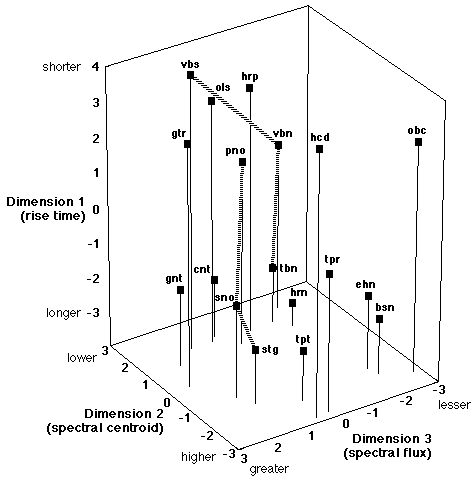
Fig. 1. Timbre space in three dimensions: a spatial model with specificities and five latent classes derived from dissimilarity ratings on 18 timbres by 88 subjects. The acoustic correlates of the perceptual dimensions are indicated in parentheses. Hashed lines connect two of the hybrid timbres (vbn and sno) to their progenitors. Two others can be examined in the same way in this figure (tpr and gnt). (See Table 1 for timbre labels.)
Estimation and analysis of class belongingness. A posteriori probabilities that each subject belonged to a given latent class were computed according to Bayes' theorem. Four subjects (three nonmusicians and one student musician) could not be unequivocally assigned to a given class as their posterior probabilities were distributed over all of the classes. They did not therefore fit into any one class and were removed from subsequent analyses of class structure. Four other subjects had ambiguous assignments to two classes with the preferred class having a probability of less than .65. The probability for the preferred class for 12 other subjects was between .65 and .95 and that for the remaining 68 subjects was greater than .95.
The distribution across latent classes of the 84 subjects for whom a preferred class could be determined was analyzed according to our original grouping by degree of musical training as well as according to three items from the questionnaire that could be conceived as ordinal scales: years of music making (composition, conducting, performance), habitual amount of music playing, and habitual amount of music listening. These data are shown in Table 5. Two of the professional musicians (one each from Classes 1 and 4) did not fill out the questionnaire and so their data are absent from the last three factors in the table.
| Musical training | Class 1 | Class 2 | Class 3 | Class 4 | Class 5 |
|---|---|---|---|---|---|
| Professional | 8 | 5 | 0 | 7 | 4 |
| Amateur | 9 | 17 | 2 | 3 | 7 |
| Nonmusician | 7 | 4 | 1 | 7 | 3 |
| Music making | Class 1 | Class 2 | Class 3 | Class 4 | Class 5 |
| >10 years | 12 | 14 | 1 | 7 | 10 |
| 5-10 years | 3 | 6 | 0 | 0 | 1 |
| 0-4 years | 8 | 6 | 2 | 9 | 3 |
| Music playing | Class 1 | Class 2 | Class 3 | Class 4 | Class 5 |
| Every day | 12 | 14 | 1 | 5 | 8 |
| Occasionally | 5 | 5 | 1 | 4 | 3 |
| None | 6 | 7 | 1 | 7 | 3 |
| Musical listening | Class 1 | Class 2 | Class 3 | Class 4 | Class 5 |
| >3 times/day | 8 | 8 | 0 | 6 | 4 |
| 2-3 times/day | 11 | 11 | 0 | 6 | 6 |
| <2 times/day | 4 | 7 | 3 | 4 | 4 |
Table 5. Distribution of subjects in each latent class according to degree of musical training, number of years of music making, amount of music playing and music listening. (The bottom panel has data for only 82 subjects since two professional musician subjects did not fill out the questionnaire.)
The musical training factor categories are defined above in the Methods section. The music making categories were defined by the number of years of musical activity. While these two factors certainly covary, we felt that they might reveal different tendencies. The music playing categories were defined by the amount of regular instrumental practice and the music listening categories by the frequency of daily listening. In the analysis, Classes 1 and 2 were combined since their weight patterns were similar and Class 3 was removed since there were too few subjects for the analysis to be reliable. A table of counts for each analysis class and category was constructed from the data in Table 5. The null hypothesis was that the proportional distribution of categories for each analysis factor is constant across classes. Differences in distribution may indicate a relation between these biographical factors and class belongingness.
An exploratory data analysis technique based on counted fractions ([Tukey, 1977, chap. 15]) was used to evaluate differences between classes for each factor. The folded log (or flog) represents the difference between the log of the proportion of data below a cutoff point between two categories on an ordinal scale and the log of the proportion above that point. This statistic is preferable for comparing classes to the raw proportion in each category as it is symmetric about a mid-point of equal proportion, due to the folding or differencing part, and increases the importance of smaller differences near the endpoints of the scale (0 and 1), due to the log transformation. This analysis shows that the distributions of categories of a given biographical factor are not the same for all classes for the factors musical training and music making, indicating differences across classes, while they are similar or parallel for the factors music playing and music listening, indicating a lack of difference. However, as can be seen in Table 5, it is generally the case that each class contains some people of each category of a given biographical factor, indicating that each category of a factor can give each of the weighting types revealed by the class structure.
The first two dimensions of our timbre space were strongly correlated with the dimensions that Krumhansl labeled "temporal envelope" and "spectral envelope". However, Krumhansl's "spectral flux" dimension was not significantly correlated with any of the dimensions in our model, suggesting differences between the subject populations for this dimension. Although the specificities were significantly correlated between the two studies (see Table 6), there were important differences between them: the harp and guitarnet had much higher specificities in Krumhansl's model than in the present one, whereas the trombone, trumpet, and trumpar had moderate specificities in the present model and specificities of zero in Krumhansl's model.
For comparison, we computed the correlations (df = 16 in all cases) between the coordinates on the common dimensions of Krumhansl's (1989) model and each of the dimensions of the six-dimensional model selected by BIC. Krumhansl's "temporal envelope" and "spectral envelope" dimensions were well correlated with dimensions 1 [r = .98, p < .0001][5] and 3 [r = .77, p < .01] of the six-dimensional space, respectively. Her "spectral flux" dimension, however, was significantly correlated with dimensions 3 [r = .60, p < .01], 4 [r = -.53, p < .05], and 6 [r = -.57, p < .05]. So our dimension 3 correlated with two of her three dimensions and her dimension 2 correlated with three of our six dimensions. The most coherent relation thus exists between the two models with three dimensions and specificities.
| Our Model | |||||
|---|---|---|---|---|---|
| Krumhansl's Model | Dim 1 | Dim 2 | Dim 3 | Dim 4 | |
| "Temporal Envelope" | .98+ | .09 | .27 | ||
| "Spectral Flux" | -.33 | -.20 | -.24 | ||
| "Spectral Envelope" | -.01 | -.95+ | -.07 | ||
| "Specificities" | .58* | ||||
Table 6. Correlations (df = 16) between coordinates in Krumhansl's (1989) and our three-dimensional models with specificities for 18 timbres.
More recently, however, Krimphoff et al. (1994) have quantified satisfactorily all three common dimensions of Krumhansl's (1989) model. The first dimension correlated very strongly [r = .94] with the logarithm of the rise time (measured from the time the amplitude envelope reaches a threshold of 2% of the maximum amplitude to the time it attains maximum amplitude). The second dimension correlated very strongly [r = .94] with the spectral centroid (measured as the average over the duration of the tone of the instantaneous spectral centroid within a running time window of 12 ms). The third dimension correlated well [r = .85] with a measure of spectral irregularity (log of the standard deviation of component amplitudes from a global spectral envelope derived from a running mean of the amplitudes of three adjacent harmonics) rather than with any of a number of measures of spectral variation over time as was presumed by Krumhansl in originally naming this dimension "spectral flux".
One of the aims of the current study was to validate the acoustic correlates described by Krimphoff ([Krimphoff 1993]; Krimphoff et al., 1994) for a timbre space based on a large set of dissimilarity ratings given by subjects with varying degrees of musical training. We therefore correlated these acoustic parameters with the coordinates of the 18 sounds (df = 16 in all cases) of the present study (see Table 7). Log attack time accounted for 88% of the variance along Dimension 1 of the perceptual model [r = -.94, p < .0001]. Spectral centroid accounted for 88% of the variance along Dimension 2 [r = -.94, p < .0001]. The third dimension (as is the case in most previous studies) presented more of a difficulty in deriving its psychophysical interpretation. The spectral irregularity measure that accounted for 72% of the variance along Krumhansl's second dimension was not significantly correlated with the third dimension in the present spatial model. The label "spectral flux" given to her third dimension would suggest a parameter measuring the degree of variation of the spectral envelope over time. One such measure developed by Krimphoff (1993) described spectral flux as the average of the correlations between amplitude spectra in adjacent time windows: the smaller the degree of variation of the spectrum over time, the higher the correlation. This parameter correlated significantly with the third dimension of our spatial model, but only accounted for 29% of the variance along this dimension [r = .54, p < .05]. The explained variance increased to 39% when four of the timbres (clarinet, trombone, guitarnet, and vibrone) were removed from the correlation [r = .63, df = 12, p < .05]. Their removal did not affect the correlations of attack time and spectral centroid with dimensions 1 and 2.
| Acoustic Correlate | Dim 1 | Dim 2 | Dim 3 |
|---|---|---|---|
| Log Attack Time | -.94+ | -.12 | -.16 |
| Spectral Centroid | -.04 | -.94+ | -.21 |
| Spectral Irregularity | .41 | .31 | .13 |
| Spectral Flux | -.07 | .13 | .54* |
Table 7. Correlations (df = 16) between acoustic parameters (Krimphoff, 1993; Krimphoff et al., 1994) and the coordinates of 18 timbres along the three common dimensions of our spatial model (five latent classes and specificities derived from dissimilarity ratings by 88 subjects).
Given the high degree of variation in duration and level among the stimuli (obtained by perceptually equalizing the sounds for loudness and subjective duration), we also correlated various measures of these parameters with the coordinates on the common dimensions. For duration, we computed the energy envelope of each sound (rms amplitude of the waveform over a 10 ms running window that advanced in 5 ms steps). The maximum point of this envelope was determined and the duration encompassing the part of the signal exceeding thresholds of 3, 10, and 20 dB below this maximum were computed. For level, we also determined the rms amplitude across the entire duration of each sound (expressed in dB). These values, as well as the total physical duration and maximum SPL recorded on a sound-level meter (see Methods section) were correlated with the coordinates of each timbre on the common dimensions. After using Bonferroni's correction for multiple tests, the only correlation that attained significance was between the -3 dB threshold duration and the coordinates of dimension 1 [r = -.82, df = 16, p < .0001]. For the set of synthesized instrument sounds used, the rise time was also strongly correlated with this duration measure [r = .82, df = 16, p < .0001]. This correlation reflects the fact that, in general, impulsive sounds tend both to have sharp attacks and to begin decaying immediately, since there is no sustained excitation of the instrument. A similar interpretation was advanced by Iverson & Krumhansl (1993) for one of their dimensions.
For comparison, we also computed the correlation of Krimphoff et al's (1994) parameters with the coordinates on the dimensions of the six-dimensional solution selected by BIC (df = 16 in all cases). An equivocal result was found here as was the case with the correlation of this high-dimensional solution with Krumhansl's (1989) model. The log rise time and spectral flux parameters correlated significantly only with dimensions 1 [r = -.94, p < .0001] and 2 [r = .51, p < .05], respectively. The spectral fine-structure parameter correlated significantly with dimensions 3 [r = -.55, p < .05], 4 [r = .68, p < .01], and 6 [r = .52, p < .05]; and the spectral centroid correlated significantly with dimensions 2 [r = -.74, p < .01] and 3 [r = -.75, p < .01]. So two of our dimensions each correlated significantly with two acoustic parameters and two of the acoustic parameters correlated with several dimensions. We conclude that the psychophysical interpretation of this high-dimensional solution is rather ambiguous compared with the three-dimensional solution.
In contrast to the six-dimensional solution, note in Table 7 that each of the acoustic parameters that correlated significantly with a given dimension of the three-dimensional model with specificities was correlated with only that dimension. This orthogonality of the acoustic parameters associated with our perceptual dimensions is what makes a psychophysical interpretation possible. Further, an analysis for three dimensions without specificities was performed to evaluate the effect of removing specificities on the correlations of the acoustic parameters with the coordinates of the resulting solutions. If the specificities were removed, the correlation of spectral centroid with dimension 2 was reduced from .94 to .79, and that for spectral flux with dimension 3 was reduced from .55 to .27. The inclusion of specificities thus improved the psychophysical interpretation of the dimensions.
A similar additional analysis for three dimensions with specificities and only one latent class was performed to evaluate the effect of removing latent class structure on the correlations of the acoustic parameters with the spatial configuration. If only one latent class was used, the correlation of spectral flux with dimension 3 was slightly reduced from .55 to .49. These results indicate that the fit of the model to acoustic variables was slightly enhanced by including latent classes.
| Instrument | Specificity | Description of distinguishing characteristics |
|---|---|---|
| Trombone | 2.1 | slightly raspy attack |
| Guitarnet | 2.1 | slight high frequency "zzzit"! on offset |
| Trumpet | 2.7 | nothing remarkable |
| Striano | 3.1 | downward pitch glide at end of tone |
| English horn | 3.5 | nasal formant, very sudden offset |
| Trumpar | 3.8 | noisy/rough attack, roughness in resonance of sound, low frequency thud on onset and offset |
| Vibraphone | 3.8 | metallic sound |
| Piano | 4.2 | slight inharmonicity and soft graininess |
| Harpsichord | 4.7 | versy sharp, pinched offset with clunk |
| Clarinet | 6.4 | hollow timbre (very distinctive) |
| Vibrone | 6.4 | wobbly double attack |
One might have imagined at the outset that hybrid instruments, being unfamiliar to listeners, would have a novelty that would distinguish them perceptually from the more traditional instruments. On average, however, the hybrid timbres do not have greater specific weights than the conventional instrument imitations, neither in Krumhansl's (1989) study nor in the present one. In fact, three of the six hybrids have lower than average specific weights. The highest specific weights found systematically in both studies were for the vibrone, the clarinet, the harpsichord, and the piano. The lowest weights in both studies were found for the obochord. The specificity of the piano-like sound argues strongly against the relation between specificity and familiarity since this instrument is probably one of the most familiar to the primarily European listeners that participated in this study. It is possible that in the case of certain instruments, such as the harpsichord, the properties suggested by the specificities are related to the simulation of specific mechanical properties of the object. In this case, the acoustic result of the return of the hopper in the harpsichord mechanism is perceptually important and should certainly play an important role in an identification task. Similarly, the timbre of the clarinet has a specific acoustic property that is related to the predominance of odd harmonics in its spectrum, due to the conical geometry of the air column.
These results suggest that subjects did indeed make dissimilarity judgments on the basis of criteria related to structural characteristics of the stimuli. Certain of these criteria incited the subjects to analyze the relatively global and common degree of dissimilarity of all the stimuli based on continuous dimensions. The goal in this case was to determine the relations among stimuli along these common dimensions. Some stimuli, though, would seem to possess certain unique structural characteristics that cannot be accounted for by the Euclidean spatial model alone. These specific features or dimensions would be sufficiently salient perceptually to influence the dissimilarity of some timbres with respect to others. An indication of the presence of such features could lead to more systematic psychophysical analyses whose orientation would be quite different from an analysis based only on a Euclidean spatial model.
Recall that Class 1/2 gave roughly equal weights across dimensions and specificities, while Classes 4 and 5, gave high weights on two dimensions, or on one dimension and the specificities, and low weights on the others, respectively. It is these patterns that our analysis sought to explain by the biographical factors. One interpretation of the patterns is that the equal weights for Class 1/2 reflect a shifting of attention among dimensions and specificities over the course of an experimental session, which averages out over trials. The subjects of Classes 4 and 5 may have adopted more consistent strategies of judgment that focussed on a smaller number of dimensions and stuck to them throughout the experimental session. Another interpretation is that members of Class 1/2 were able to focus on more dimensions at a time than could the members of the other classes, and one might predict a priori that these would be principally musicians. At any rate, the factor responsible for making Class 4 focus on the attack time dimension and the specificities, while Class 5 focussed on the spectral centroid and spectral flux dimensions is difficult to tease out from the analysis of the biographical factors presented in the Results section. Overall, both musicians and nonmusicians were able either to weight all dimensions equally (Classes 1 and 2) or to give special attention to some dimensions (Classes 4 and 5). Nor does the degree of musicianship or amount of training, playing or listening mean that one factor or another will be given preferential weight. The pattern of weighting of a given subject cannot be simply predicted from the biographical data related to that subject. It would thus seem difficult to extract any clear picture of the factors influencing the weight patterns from biographical factors related to musical training and activity.
Separate CLASCAL analyses (three dimensions with specificities and one latent class) were performed for the professional and nonmusician groups as well as for each individual latent class. The variance about the model distances was much greater for the nonmusicians (3.53) and amateurs (3.64) than for the professionals (2.75). The variances for the individual latent classes (containing mixtures of professionals, amateurs, and nonmusicians) were less than the variance for the professional group (range 2.41-2.72). The inclusion of class weights in the dimensional model is thus justified in terms of model fit since it reduces the overall variance. This pattern of results suggests that the effect of musicianship is, among other things, one of variance. Latent classes do not differ with respect to variance, but musicians and nonmusicians do. So musicianship affects judgment precision and coherence.
The CLASCAL analysis suggested a six-dimensional model without specificities for individual timbres with a three-dimensional model with specificities being a close contender. Psychophysical quantification of the three-dimensional model was achieved, whereas only one dimension of the six-dimensional solution was unequivocally correlated with one of the acoustic parameters derived by Krimphoff (1993; Krimphoff et al., 1994). Further, the first two dimensions and the specificities of the three-dimensional model correlated significantly with a similar spatial solution found by Krumhansl (1989), who employed a group of professional musician subjects and a set of stimuli including all of ours.
The acoustic correlates of the three common dimensions in our spatial model were log rise time, spectral centroid, and spectral flux. The first dimensions was also well correlated with the duration during which the sound's amplitude envelope remained within 3 dB of the maximum, suggesting that this dimension distinguishes impulsively from continuously excited sound sources. In most multidimensional scaling studies of musical timbre, dimensions qualitatively related to the first two parameters have been found. The third dimension seems to be less stable across subject populations (comparing this study with that of Krumhansl, 1989) and/or stimulus sets ([Grey, 1977]; [Grey & Gordon, 1978]; Krimphoff et al., 1994).
That abstract parameters such as spectral centroid, spectral irregularity, and spectral flux seem to explain some of the dimensions used to compare timbres in a dissimilarity rating task, may suggest that such judgments are based in part on raw sensory qualities. A dimension related to the manner of excitation of the instrument would suggest that the judgments also include inferences about the nature of the sound sources involved. According to this view, differences between latent classes of subjects would reflect differences either in sensitivity to these qualities or in the importance accorded to them in the comparisons made by the subjects. This notion is further supported by the fact that similar predictive variables are found for synthetic sounds of varying degrees of resemblance to acoustic sources (Miller & Carterette, 1975; the present study), for recorded instrument tones ([Iverson & Krumhansl, 1993]; [Serafini, 1993]; [Wedin & Goude, 1972]), or for analyzed, modified, and resynthesized instrument tones ([Grey, 1977]; [Grey & Gordon, 1978]; [Iverson & Krumhansl, 1993]). Nonetheless, none of these studies really presented a broad and balanced set of instrument sounds that derive both from different types of resonating structures (strings, bars, plates, air columns) and means of excitation (blowing, bowing, striking, plucking). Such a set would allow systematic variation of the many types of physical properties that instruments possess, perhaps giving rise to judgments of a more classificatory than continuous nature. Work in progress in our laboratory intends to clarify this issue.
The specificities that were suggested by the model were explored informally in the present study. This exploration suggested that distinguishing features of the timbres that are indicated by the specificities in the CLASCAL analysis are of two types: additional perceptual dimensions on which only certain sounds vary, and discrete features that are of varying degrees of perceptual salience. Further work in both acoustic analysis and psychophysical experimentation is needed to verify and develop this notion.
The CLASCAL algorithm (Winsberg & De Soete, 1993), and in particular the extended version employed here, promises to be a powerful tool for the analysis of timbre perception. Specificities are a way of representing systematic variation in dissimilarities that can't be accounted for by shared dimensions, and they may indicate additional dimensions along which only a single or a small number of timbres vary or unique attributes with varying degrees of perceptual salience. Further, the model captures certain systematic variations in judgments that are accounted for by differential weighting of the common dimensions and the specificities by latent classes of subjects. Taken together, these added modeling features give a better fit to the data and render the resulting model more interpretable in terms of its acoustic correlates. This approach provides a much needed tool for the analysis of complex perceptual representations and for suggesting orientations for their psychophysical quantification.
Acknowledgments. The authors would like to thank Eric F. Clarke for help in recruiting subjects at the Music Department, City University, London, U.K. and two anonymous reviewers for helpful comments.
____________________________
Server © IRCAM-CGP, 1996-2008 - file updated on .
____________________________
Serveur © IRCAM-CGP, 1996-2008 - document mis à jour le .