Tous droits réservés pour tous pays. All rights reserved.
| Serveur © IRCAM - CENTRE POMPIDOU 1996-2005. Tous droits réservés pour tous pays. All rights reserved. |
The computer simulation of room reverberation has been shown to be of importance in the fields of computer music, architecture, and acoustics. The research described herein covers the use of recirculating delays to produce sounds like those of room reverberation, and the actual simulation of room acoustics by the phantom source method. To these ends, several new forms of recirculating delay reverberators were tested with the results that a comb filter with a low-pass filter in the loop produced results most consonant with the sounds of actual rooms. The low pass filter helps simulate the low-pass filtering effect of the air on the sound transmission in the room. It is later shown that no system consisting only of recirculating delays can reproduce exactly the response of a real room except in certain highly degenerate cases. An improvement is suggested using the simulated impulse response of the room for the early echos and recirculating delays for the late response. This provides the most satisfactory and natural sounding reverberation to date. A program was constructed to simulate the impulse response of natural rooms with certain geometrical restrictions. This program was used to gain insight into the process of reverberation and also to attempt to simulate exactly the early reverberation of a given hypothetical concert hall. Suggestions are made for the further improvement of the artificial reverberation, plus a design technique for artificial reverberation is given.
When music is performed in a concert hall, a torrent of echos from the various different surfaces in the room strike the ear, producing the impression of space to the listener. This effect can vary in evoked subjective response from great annoyance or even incomprehensibility in the case of speech presented in a highly reverberant auditorium to sheer ecstacy in the case of late romantic music in the Vienna Grosser Musikveriensaal. Most music is heard these days either in the comfort of one's home (or car), or in a university auditorium, both of which have generally short reverberation times. For this reason, most recordings of music already have some amount of reverberation added before distribution either by a natural process (ie. recordings taken in concert halls) or by artificial processes (plate or spring reverberators). Computer music is an especially fertile ground for artificial reverberation in that it is rarely, if ever, performed in highly reverberant concert halls. The use of the computer for the simulation of this reverberation also allows the composer another degree of freedom, namely to "tailor" the reverberation to the particular aural effect he wishes to present, allowing, for instance, each individual sound in the piece to carry an entirely different spacial aspect, if desired. In this paper, we review some of the work that has been done in the production of artificial reverberation by computer and we present the fruits of our own labors along this line, both in the attempted simulation of the concert hall environment by computer and in the proliferation of different circuits for realization of simulated room reverberation.
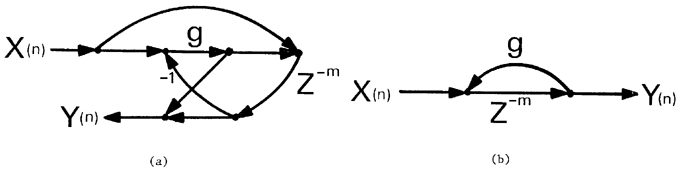
Although the study of acoustics may have started as early as the 6th century B.C. with Pythagoras' inquiries into the discovery that halving the length of a string seemed to double its pitch, our own treatment will begin with the first published computer simulations of room reverberation by Schroeder (1961, 1962). We will not have time to discuss directly the first published study of room reverberation by Sabine (1972) (published originally in 1900, reprinted in 1972). The two systems proposed by Schroeder are combinations of two unit reverberators, shown in cannonical form in figure 1. The first one is the all-pass filter, shown in figure 1b in the 1-multiply form. The second is the comb filter in figure 1a.
We should say a quick word about our use of signal flow graphs to represent filter structures. In our formulation, X always represents the input to a filter and Y always represents the output. An arc of a graph which is not labeled is a unity gain arc. Sometimes we insert extra nodes for supposed clarity. More than one arc coming together at a node are to be summed. A node with several arcs leaving supplies the same identical signal on all arcs leaving the node. An arc can be a gain (a multiply), a delay (denoted by Z, the unit advance operator, raised to a negative power), or another filter, usually represented by a capital letter as a function of z.
To continue with our exposition, the unit reverberators shown in figure 1 have, by themselves, the following transfer functions :
1)
2)
Figure 1
The simplest unit reverberators (a) 1-multiply all-pass (b) comb filter. The magnitude of g must be less than one for stability.
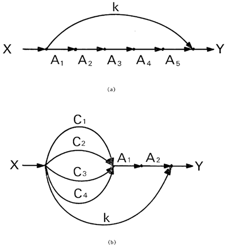
Figure 2
Combinations of unit reverberators to make a functioning reverberator. In each combination, the direct signal is added in with a scaling of k. (a) Series connection of all-pass networks. The functional dependence on z has been dropped in the illustration. (b) Parallel combination of comb filters followed by series combination of all-pass filters.
It is simple to show that the transfer function in equation (1) is indeed that of an all-pass filter, in that the coefficients in the numerator are in reverse order of those in the denominator, thus forcing the zeros to be the reciprocals of the poles. This is sufficient for the filter to be an all-pass. We must remember, however, that the all-pass nature is more of a theoretical result than a perceptual one. We should not assume that simply because the frequency response is absolutely uniform that the filter is perceptually transparent. In fact, the phase response of the all-pass filter can be quite complex. The all-pass nature only implies that in the long-run, with steady-state sounds, the spectral balance will not be changed. This implies nothing of the sort in the short-term, transient regions. In fact, both the all-pass and the comb filter have very definite and distinct "sounds" that to the experienced ear can be immediately recognised.
To use these as a reverberation generator, we must combine them in some manner. Schroeder suggested two different combinations, shown in figures 2a and 2b. In these figures, Ai represents an all-pass filter and Ci represents a comb filter. Figure 2a thus shows a series connection of all-pass filters with a final addition of some proportion of the original signal. With the all-pass, there is also a feed-through of the original signal scaled by the gain, g, of the all-pass, so with the circuit of figure 2a, we will find a total direct signal contribution of one plus the product of the gains of the individual all-passes. In 2b, we see a parallel connection of four comb filters followed by two all-passes, with again a feed-forward connection of a proportion of the original signal. The idea with both of these is to use the unit reverberators to simulate the effect of wall reflections and transit time of the wave front as it passes from one wall to the other. The addition of the direct signal simulates the proximity of the source to the destination. As the destination listener moves away from the sound source, the reverberation he hears remains at about the same amplitude, but the direct sound intensity decreases by the usual reciprocal distance squared term, thus there is a distance at which the direct and reverberant sounds are equal in amplitude, such that at larger distances than this, the reverberant sound field dominates. In these circuits, we attempt to simulate the wall reflections with the feedback paths and the transit time between reflections with the delay lengths. We shall see later that this is a somewhat crude way to simulate actual rooms. Both Schroeder and this author have proposed refinements (with corresponding increases in computer time required).
In any case, the use of the reverberators in figures 2a and 2b implies that the various parameters (gains and delay lengths) of all the unit reverberators must be chosen somehow. It is generally thought important to make all the delay lengths mutually prime, in that this reduces the effect of many peaks piling up on the same sample, thus leading to a more dense and uniform decay.
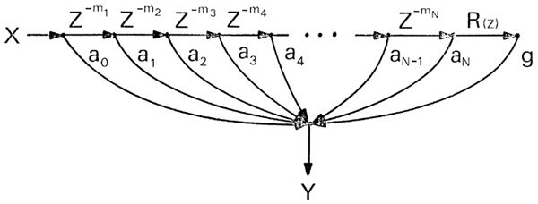
More recently, Schroeder (1970) reported on a way of simulating room reverberation taking into account the exact geometry of the room. This study involves the simulation of the source as an omnidirectional pulsating circle (the study was done in 2 dimensions), following the paths of some 300 individual rays that are cast at equally spaced angles about the source. The presumptive linearity of the air and walls makes it possible to transmit a single ideal impulse, thus obtaining the impulse response of the simulated room. The impulse response can then be convolved with musical sound to produce the sound of that music in that room. Following this, he suggested that a new reverberator could be made that simulates exactly the first few echos, then simulates the later echos by means of a reverberator such as has been shown above. This design is shown in figure 3. The first delays and gains are chosen following the geometry of the room, then the reverberator, R(z), is chosen to simulate the decay of the room reverberation after the density has reached the level where the individual pulses cannot be separated. We will come back to this idea later.
Figure 3
Form suggested by Schroeder (1970) for simulation of early echos by direct summation, using a standard reverberator as shown in figure 2a or 2b for the late echos.
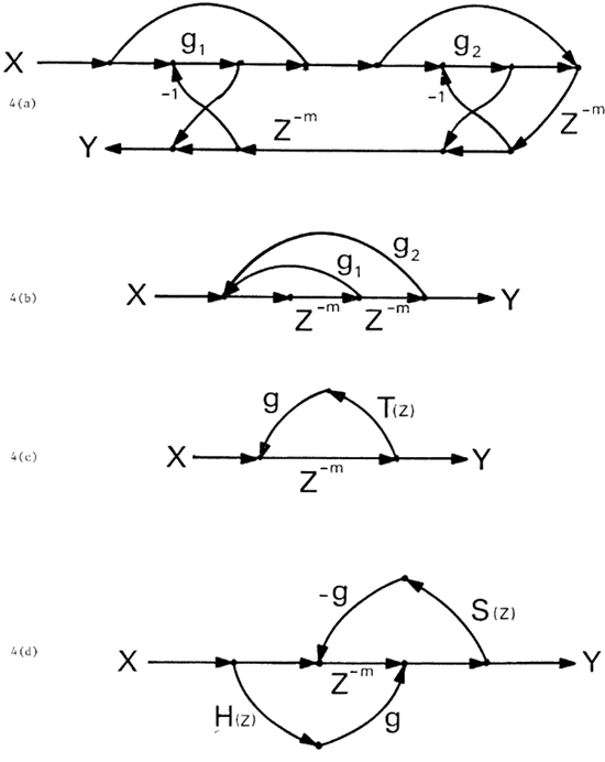
In the course of studying the art of making artificial reverberation, we have explored several new unit generators. These include the oscillatory all-pass in figure 4a. In addition, we may also replace the gain terms with filters to produce decays the lengths of which depend upon the frequency. For the non-oscillatory case, these are shown in general form in 4d for the all-pass and in 4c for the comb. There exist straightforward extensions to the oscillatory cases of comb and allpass for these configurations also. What must be discussed now is what the general utility of these units are and when they should be used. In fact, we have found that the only really useful one is the comb form in figure 4c, but we include a discussion of the others for completeness and additional insight as to the problems involved. These reverberators are all modifications of Schroeder's original designs (Schroeder, 1961, 1962), and can all be described as various forms of recirculating delays, since they all use delays with feedback and sometimes feedforward. We should point out that these units were known as early as 1966 when H. Date and Y. Tozuka (1966) simulated these units using analog filters and a variable-speed multi-head tape recorder for delay. Needless to say, the filter realizations were somewhat complex.
Figure 4
Some new unit reverberators. (a) is an oscillatory all-pass. (b) is an oscillatory comb. The impulse response of the oscillatory units is a train of pulses the amplitudes of which correspond to a decaying sinusoid. (c) is a comb filter with another filter inside the loop, identified by its transfer function T(z). (d) is an all-pass with filters in the loops identified by their transfer functions : H(z) in the feed-forward path and S(z) in the feed-back path. For this to remain all-pass, these filters must be complex conjugates of each other.
The reverberators in figures 2a and 2b have been used extensively at Stanford University, at IRCAM, and many other sites around the world in varying different configurations. With the all-pass reverberator of 2a, several problems were noticed by this author along with L. Rush, D.G. Loy, K. Shoemake, J. Chowning and others :
Although the reverberator of 2b did not show exactly these same problems, it shows other problems, namely :
Our first thought to help this situation was to try the oscillatory networks shown in figures 4a and 4b. The transfer functions of these two unit reverberators are then as follows :
3)
4)
Both these units can be described completely by the decay rate of the exponential envelope and the frequency of the oscillation. The decay rate, r, is the factor by which the amplitude is diminished every m samples (in the impulse response). The frequency, , is that of the sinusoidal part of the decay. In the case of the oscillatory comb, we can compute the coefficients g1 and g2 from the frequency and decay rate as follows :
5)
6)
Negative decay rates can also be used, making each pulse of the impulse response alternate in sign. The condition for stability is that the magnitude of r must be less than one. We can now design with the oscillatory comb just the way we have with the simple comb, with r taking the logical place of g, and with one more parameter to choose. The frequency, , is divided by m in the equation because of the delay in m samples between each pulse in the impulse response.
We can likewise compute the coefficients of the oscillatory all-pass from the desired decay rate and frequency as follows :
7)
8)
In the case of the all-all-pass reverberator, such as is shown in figure 2a, the use of the oscillatory all-pass made little or no perceptible difference, even when all units were so modified. There was a slight difference in the tail end of the decay in that the dominance of one pitch over another kept shifting so that we heard the pitch of one delay for a short while, then the pitch of another delay, and so on.
With the combination comb-all-pass reverberator, such as is shown in figure 2b, the use of oscillatory combs did help the decay a bit in the same way as with the all-all-pass case, but did not correct the principal problem, which was the response to short, impulsive sounds. The improvement is enough, however, to say that short of placing a filter in the loop, which will be discussed subsequently, the comb-all-pass reverberator with oscillatory combs was the best sounding reverberator up to this point.
Figure 4c and 4d show unit reverberators with filters in the loops. Figure 4c shows a comb-type and 4d can be made an all-pass with the proper choices of the filters H(z) and S(z). For the filter to be all-pass, the loop filters H(z) and S(z) must be complex conjugate. This implies that their impulse responses are the time reverse of each other. Since the feed-forward filter, H(z), passes directly into the output, it should be unconditionally stable. This gives us the entertaining result that either H(z) and S(z) must be FIR filters, or S(z) must be an unstable filter when viewed in isolation. Strangely enough, if the magnitude of S(z) when evaluated on the unit circle is everywhere less than unity, the unit reverberato as a whole will be stable (see below). This notwithstanding, we consider it a somewhat bad idea to put an unstable filter in the loop because the delay of m samples prevents any annihilation of the response of SW for a certain time, during which time, the response of S(z) may well have exceeded the bounds of the computer on which it is being run. For this reason, we consider it more reasonable to use FIR filters for H(z) and S(z). To make the circuit realizable, we must insert a delay after the node where the feedforward path breaks off of the original signal and before the node where the feedback path adds into the original signal, a delay equal to the total delay of the feedforward filter H(z). Some additional efficiency can be obtained by the use of linear phase filters here.
The purpose of placing a filter in the loop is to help simulate the effect of the attenuation of the higher frequencies by the air. This attenuation is due "partly to the effects of viscosity and heat conduction in the gas and partly from the effects of molecular absorption and dispersion in polyatomic gases involving an exchange of translational and vibrational energy between colliding molecules". (This description lifted with minor paraphrasing from Beranek (1954)). Unfortunately, we have found much disagreement in the literature as to exactly what these constants are. The reported values vary by as much as a factor of five in the decay rate. In any case, the intensity of the sound is generally thought to vary, for any given frequency, according to the following formula :
8)
Where Io is the intensity at the source, x is the distance from the source in meters, and m is the attenuation constant which depends on both frequency, humidity, pressure, and temperature. Table T was taken from Kuttruff (1973) who claims to have taken it from Harris (1964) and Harris and Tempest (1964). The absorption seems to go up even higher at lower values of humidity, and at higher frequencies. These absorption coefficients may not seem very high, but in a large concert hall such as the Boston Symphony Hall, the reverberation time of more than 1.7 seconds implies that the sound has traveled more than 600 meters in traveling between the various walls. This would mean (at 40 percent relative humidity, a typical figure in the Boston area during the concert season) that the 4 KHz signals would have been attenuated upwards of 60 dB more than the 1 KHz signals. This just shows that this process is significant and cannot help but have a substantial effect on the resulting spectrum of the late decay. Now we can approach the question of modifying the unit reverberators to simulate this facet of sound transmission. We must keep in mind, however, certain perceptual relations in reverberation that have been noticed over the years. During the performance of a passage of music, only the first 10 or 20 dB of the decay of the reverberation is typically audible because of the changing nature of the music. It is only in pauses or ends of movements where the entire decay of the reverberant sound will be audible. It is not clear what this fact implies except perhaps that we must concentrate equally on the early decay and the late decay for a comprehensive simulation.
Since one problem that arises immediately with the new unit generators is that of the stability of the resulting unit when one inserts a filter into the feedback loop, it is important to take a closer look at the stability conditions for such filters.
We can compute the stability of the comb by carrying the transfer function of the filter that has been inserted in the loop along explicitly, then separating it into its magnitude and phase functions as follows :
9)
This then has as magnitude function, evaluated on the unit circle :
where |T| is the magnitude of and is the angle of . is the radian frequency around the unit circle and Ps the sampling period in seconds. Ignoring for a moment the angular term, we can see that |T| follows g around at each point in the formula. This implies that we can consider the effect of the filter separately on the radii of the roots and on their angular placement. Without the filter, the roots are placed evenly at multiples of the frequency 1/m Ps and at a uniform radius of g. With the filter, the radii have been changed to g|T| which depends on the input frequency, , and the angular position has been distorted to the following :
11) for i = 0, 1, 2, ....
For stability, all we need to do is assure that the radius never reaches 1.0, so the condition for stability becomes this :
Thus knowing the absolute maximum value of |T|, we can easily scale g to be unconditionally less than the reciprocal of this. This guarantees stability.
Figure 5
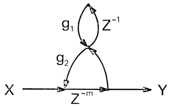
One form of the comb with a filter in the loop as shown in figure 4c. Here we have chosen a simple 1-pole filter. If g1 is positive, it will be a low-pass filter. For stability, g2 (1 - g1) must be of magnitude less than one.
To test this idea, the filter shown in figure 5 was incorporated into a reverberator of the form shown in figure 2b. The loop filter is a simple first-order filter. For stability, the magnitude of g1 should be less than one. If we insist that the loop filter be strictly low-pass, then g1 should also be positive, and the maximum of |T| will occur at , as is shown by its transfer function :
13)
and its maximum value at will be :
14)
Thus if we set g2 to g(1 - g1), where g is now between zero and one as before, the resulting filter is unconditionally stable and has the side benefit of giving us a parameter in the familiar zero to one range.
Again, the idea of inserting such a filter in the loop is to simulate the absorption of the high frequencies by the air. The frequency response of such a simple low-pass filter as that shown in figure 5 can never conform to the spectral modification necessary to exactly simulate this property but was chosen as a compromise with efficiency, since it only adds one multiplication. There is a question, however, of how to set this parameter, g, which controls the roll-off of the filter. To this end, a series of optimisations were done, using the Marquardt algorithm (Marquardt 1963) to match the frequency response of this low-pass filter in a least-magnitude-squared manner to the actual data reported in the literature. The results are summarized in Table 1. The resulting optimal values of g1 are shown in figure 6. Unfortunately the values are strongly dependent on sampling frequency and somewhat dependent on humidity, temperature and pressure. The figures are given here for sampling rates of 10 KHz, 25 KHz, and 50 KHz at four different values of humidity. Again, the weakness of the first-order filter as a low-pass means that these can only be considered very vague approximations of the actual sound absorption of air, so the exact value of this coefficient should not be taken too seriously. These should only be considered guideline values.
Following these guidelines, we can choose a value for the low-pass filter coefficient that represents the attenuation that a specific delay will produce. Whatever delay that we choose for this comb, we can convert that delay into meters by multiplying by the speed of sound in air, which is generally taken to be 344.8 meters per second at 22 degrees Centigrade and standard pressure of 751 millimeters of Mercury. For the appropriate value of humidity and sampling rate we can read off directly the value of g1 from the graphs of figure 6. For intermediate sampling rates, an interpolation can be done.
Following this procedure indeed produces a reverberation such that the decay of the higher frequencies is somewhat faster than that of the lower frequencies, and indeed, the resulting sound is somewhat more realistic. Several other benefits immediately occur also, such as the loss of sensitivity to the exact delay length and a more robust treatment of short, impulsive sounds. The configuration we have been favoring is that with 6 comb filters, each with low-pass filters in the loop, and 1 single all-pass filter.
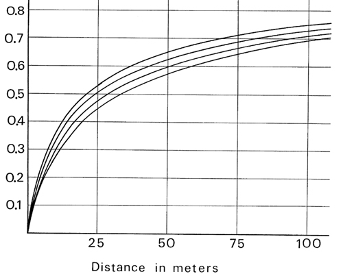
Figure 6
Graphs of the optimal gain, g1, of the low pass filter in the feedback loop of a comb filter as shown in figure 5 for simulating as well as possible the natural high frequency attenuation of the air. Figure 6a is for a sampling rate of 10 KHz, figure 6b for 25 KHz, and 6c for 50KHz. The delay length must be converted to meters, then for the appropriate humidity (higher on the east coast), the value of the coefficient can be read off directly. For intermediate sampling rates or humidities, an interpolation must be done. Since this value is not highly critical, no special care must be taken with such an interpolation.
Beranek (1963) reports that for "good" bass quality in a concert hall, it should have a ratio of the reverberation time at 125 Hertz and the mid frequency reverberation time (average of the 500 and 1 000 Hz reverberation times) of somewhat greater than unity. The comb of figure 5 exhibits exactly this property for any positive value of g1. Specifically, for the values of g1 in figure 6, the ratio is around 1.02, which is designated by Beranek as customary in a "good" concert hall. This point is actually somewhat moot in the computer music domain, in that the reason that bass is to be emphasized in concert halls is that string basses are somewhat weak, especially when one considers the lack of sensitivity of the ear to lower frequencies, such that they must be amplified by the room itself if possible to balance properly with the orchestra.
We have found that in the use of the 6 comb reverberator, certain distributions of values make more sense than others. For instance, with more than 6 combs or more than 1 all-pass, the difference in sound quality is largely unnoticable. The delays seem to work well when distributed linearly over a ratio of 1:1.5 with all the g1 terms set to a constant number g times (1 - g1). The all-pass seems to work well at about a 6 millisecond delay and a gain of 0.7 or so. As a concrete example, Table II shows the values of delays and low-pass filter gains for such a reverberator at 25 KHz sampling rate and at 50 KHz. Again, the loop gains, g2 should be set to a number, g, times (1 - g1) for each comb. Each comb will have a different value of g, but should have all the same value for g. This number, g, determines the overall reverberation time. For example, values around 0.83 seem to give a reverberation time of about 2.0 seconds with these delays.
The distribution of these numbers, g, for the combs determines the dominance of one comb over another in the decay. If one notices that a particular comb's pitch is dominating the decay, the value of g for that comb can be reduced. With less than 6 combs, one can never arrive at a set of values of g that mask entirely the dominance of a particular comb.
Additionally, the all-pass seems to be a somewhat sensitive subject too, in that too short a delay for the all-pass gives an annoying "puff-puff" response to background noise. If there are any clicks or pops in the sound being reverberated, a short all-pass will surround each click with a "puff" consisting of its own impulse response, sounding not unlike a very quiet cymbal crash. To eliminate this kind of sensitivity, the shorter delays should be avoided. A further complication, however, is that any longer delay than 6 milliseconds seems to produce an audible repetition period, thus the delay of the all-pass is pretty well limited to 6 milliseconds.
Turning now to the reverberator as a whole, we have tested this formulation with delays as short as 10 to 15 milliseconds for the combs with the results that the sound is still good, and that long reverberation times can still be obtained even with such short delays. The subjective impression of the simulated concert hall changes in this case such that at the shorter values of delay, one might well imagine that one were inside a garbage can rather than the Symphony Hall, but the density and "naturalness" is still good, although one might quarrel with the subjective impression of the timbre.
Indeed, this seems to be about as good as one can do with the recirculating delay system of reverberation. It does not seem to add anything by putting more complicated filters in the loop, except that one can then simulate other architectural decisions, such as the composition of the walls or the absorption of an audience. The low-pass filter in the loop seems to help the response to short, impulsive sounds by smearing out the echos. Each echo is no longer a discrete impulse, but is lengthened by the simulated transmission characteristics of the air itself, so that even in the early reverberation period with its correspondingly lower density, the discrete echos seem to be effectively masked. It likewise did not seem to add anything to use the all-pass network with the filters in the loop (figure 4d), so this unit does not appear useful.
We might mention here that it is not absolutely necessary to set the values of g1 from the optimal values shown in figure 6. One can just set the values arbitrarily to produce different kinds of sounds that have little or no relation to physical reality. Larger values of g1 produce a reverberation with a very bright beginning and a very muffled decay. Small values of g1 tend toward the case where there is no filter in the loop. The use of different values of g1 for different combs produces no particularly different sound, but can cause dominance on one comb over the others.
We should add here a quick word about implementation. Normally, these reverberation schemes will be implemented either on special-purpose digital hardware or on general-purpose computers. In either case, one should pay special attention to the error characteristics of these reverberators, as this is important with all types of filters. Following the formulation of Oppenheim (Oppenheim and Weinstein 1972, Oppenheim and Schafer 1975), we can approximate the error amplification of the reverberator of figure 5 as 1/(1 - g). Likewise, the signal itself can be amplified by that same factor. For example, if g = .75, then we can expect the quantization error of the input signal to be increased by about a factor of 4. This would imply that we should keep two or more extra low-order bits in the computation so that this error would be truncated at the output. Likewise, we would have to keep two extra high-order bits to assure that the total dynamic range did not exceed the word length of the machine. This implies that, for instance, to get 12 good bits of output, one would have to do the intermediate computations with 14 to 16 bits, or more. Likewise, to get 16 good bits of output, one would need even more bits internally. This is improved a bit when we consider that generally the reverberated signal will be attenuated before it is added into the output, but in any case, one cannot afford to ignore the effects of finite register length in the implementation.
If this were not enough, there is a further phenomenon that occurs with fixed-point implementation of digital filters : that of limit cycles. Depending on the type of arithmetic used (rounding, truncation, etc) the output of the filter (reverberator) may not descend exactly to zero even after the input has vanished. Output values of 1 in the last bit, or sequences of +1 and -1 are quite common in fixed point. This last case of alternating sign is especially annoying, because in 2's complement arithmetic, truncating the low-order bits does not cure the problem. Again it is not a particularly disasterous effect, but one should not be surprised when it happens.
Table I
Relative humidity Frequency in Hertz 1000 2000 3000 4000 40 .0013 .0037 .0069 .0242 50 .0013 .0027 .0060 .0207 60 .0013 .0027 .0055 .0169 70 .0013 .0027 .0050 .0145 Now the same table in units of dB per meter.
Relative humidity Frequency in Hertz 1000 2000 3000 4000 40 .0056 .0161 .0300 .1051 50 .0056 .0117 .0261 .0899 60 .0056 .0117 .0239 .0734 70 .0056 .0117 .0217 .0630
Table II
Examples of parameters for actual reverberators of the type shown in figure 2b, using 6 comb filters with the low-pass filters in the loop, such as shown in figure 5, and one standard all-pass following, as shown in figure 1a.
25 Khz 25 Khz Delay (in ms.) g1 g1 COMB 1 50 0.24 0.46 COMB 2 56 0.26 0.48 COMB 3 61 0.28 0.50 COMB 4 68 0.29 0.52 COMB 5 72 0.30 0.53 COMB 6 78 0.32 0.55 In each of these cases, the all-pass should be set to a 6 millisecond delay with a gain of 0.7 or so.
The only problem with these systems of recirculating delays is that they can never correspond to the room reflection pattern in a real room. This is because the reflections in a room, even a square one, do not typically come in regular sequences separated by equal amounts of time. To see why this should be so, we have to take a brief look at the science of room acoustics. Since we do not have room here to expound at length on the subject (the interested and brave reader is referred to one of the many introductory texts on the subject, such as Beranek (1954) or Kuttruff (1973)), we will only describe a small corner of what is called geometric acoustics.
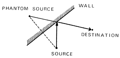
Much as in the study of light, we can keep track of the reflections in a manner that depends only on the position of the source and not on the position of the destination listener. To compute the actual impulse response of the room, we must specify the position of the destination listener, but using the method of phantom sources, we can keep track of the reflections independent of the position of the listener up until the last moment. To see how this works, let us turn to figure 7, wherein we see a simplified case consisting of one wall, one source, and one destination. In the case shown, direct sound ommitted, the wave reflects off the wall and strikes the destination. This is equivalent in effect to the case where the wall does not exist and there is another identical source that spoke at the same time as the true source. This "phantom" source is located on a line connecting the destination point and the reflection point. We may also locate the phantom source by drawing a line from the source that is perpendicular an equal distance on the other side of the wall. Thus if we now consider a room with three walls, shown in figure 8a, we can trace the various phantom sources given only the position of the source and the room geometry. In doing this for a two-dimensional room, we are assuming that the floor and ceiling are infinitely absorbing the thus do not reflect. We see that the phantom sources are represented by their bounce number. Each first bounce phantom source reflects off the other two walls to make six "second-bounce" sources. Figure 8b shows an ensemble of phantom sources up to the 5th bounce.
Figure 7 Diagram of a sound ray going from a sound source to a destination listener via a wall reflection. Just as in the case of light, we can think of the reflected sound as originating from a "phantom" source which is behind the wall, located on a line from the source that is perpendicular to the wall.
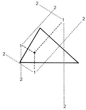
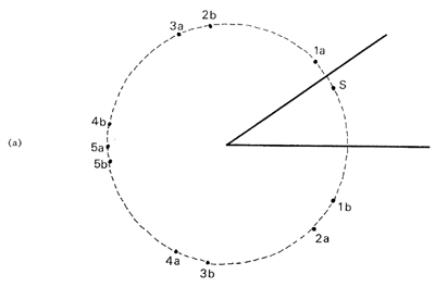
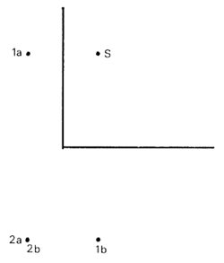
To give some slight additional insight into how these phantom sources work, we can consider the case of a corner in isolation such as shown in figure 9a. In this case, all the phantom sources will be located on a circle the radius of which is the distance from the source to the vertex. In a corner, there will only be a finite number of reflections. A phantom source cannot reflect off a wall which it is behind (obviously !). Thus, as we follow the reflections in figure 9a starting with the reflection off the upper wall, we find phantom sources at positions 1a, 2a, 3a, 4a, and 5a, the number corresponding to the number of bounces. Likewise, starting with the lower wall, we find the phantom sources 1b, 2b, 3b, 4b, and 5b, after which the phantom source is behind the wall which it would reflect off of, thus terminating the sequence. We can also see in figure 9b, the well-known case of a right angle where there are exactly 3 phantom sources, of which 2 are first bounce sources and the third is a second bounce source which receives contributions from both the first bounce sources. With any angle greater than 90 degrees, any given corner will only create two phantom sources.
Figure 8a
Patterns of phantom sources for two room shapes. (a) First and second bounce phantom sources with the perpendiculars of construction shown.
Figure 8b
Pattern of phantoms up to the fifth bounce. Note that even though there are no parallel walls, the phantom sources show very regular patterns.
Figure 9a
The phantom sources in a corner fall in a circle the center of which is the vertex of the corner. In (a) we can trace 5 phantoms which start with the first reflection off the upper wall, which are labeled 1a, 2a, 4a, and 5a. Likewise, there are 5 phantoms starting with an initial reflection off the bottom wass, which are labeled 1b, 2b, 3b, 4b, and 5b.
Figure 9b
(b) shows a rectangular corner, wherein the phantom sources number only 3, one of which is a superposition of the two-bounce sources from each wall.
We can easily write a computer program to keep track of these phantom sources. To do so, at least for rooms which are convex polygons, we only need to keep track of the locations of the phantom sources, and be able to determine whether the phantom source is in front of or behind a given wall when we are computing new phantom sources. To review our coordinate geometry a bit, let us recall that the normal form for a line in the Euclidian plane is the following :
15)
where is the inclination of the line and is the perpendicular distance from the line to the origin. Given the endpoints of a line as (X0, Y0) and (X1, Y1), we can determine the equation for the line as follows :
16)
17)
18)
Now that the line is in normal form, we can test any given point (Xt, Xt) to determine which side of the line it is on. That is,
means that (Xt, Yt) is on one side of the line, whereas
means that (Xt, Yt) is on the other.
We notice that with the normal equations for a line, there is always an ambiguity. We can always add to the angle and negate giving a different equation for the same line. This is less of an ambiguity than a fortunate extra degree of freedom, for we can use this to orient the wall equations in a standard way such that for any point, (Xt, Yt), that is inside the polygon (again, assuming convexity) with N walls whose equations are determined by and , for i = 1,..., N, the following will be true :
19) for i=1, 2, ... n
All we need to do to allow us to use this simple test is to go through the wall equations with any one point, (Xd, Yd), that is known to be inside the polygon and flip any equation for which the above does not hold. For a convex polygon, we can construct such an "internal" point by averaging the X and Y coordinates (separately, thank you) of all the vertices.
Given the normal equations for the wall lines, we can now decide : whether a given source will reflect off a given wall just by verifying that the above condition is satisfied for the appropriate value of i.
Continuing in this manner, we can compute the position of the new phantom source just by taking the equation of a line going through the originating source (phantom or not) that is perpendicular to the wall. If the equation of the wall is as shown in equation (15), then such a line is given by the following equation :
where (Xs, Ys) are the coordinates of the originating source. If we then intersect this with the wall line, we can find the coordinates of the intersection (Yx, Yx) as the following :
Thus the differences in the coordinates is simply this :
and the coordinates of the new phantom source on the other side of the wall is just the following :
Now that we know how to keep track of the sources, we must see how this affects the listener. There are three main sources of attenuation of the sound from a phantom source. The first is that each bounce presumably reduces the amplitude a bit. Wall reflection characteristics are actually very complex, depending on both the frequency and the angle of incidence of the wave front. We will brush aside this nasty intrusion of nature and for the time being represent the attenuation of each wall by a single number, the reflection coefficient. Another source of attenuation is just the fact that any spherical wave is diminished by distance at a rate proportional to the reciprocal of the distance it has travelled (note that we are working in amplitude here and not intensity. For intensity, it is the reciprocal of the distance squared). The last source of attenuation is that of the air itself which we have already discussed in the previous section.
If we ignore for one second the frequency dependence of everything, then we see that it should be quite straightforward to compute the contribution to the listener from each phantom source. We must only assure ourselves that the ray from the phantom source to the listener crosses the wall that produced the phantom source. Otherwise, the listener would not be able to "see" that phantom source. Thus at each step, we can compute the effect at the listener by adding up the contributions of all the phantom sources.
A program was written here at IRCAM for examining 2-dimensional convex polygonal rooms using this simplified phantom source model. The procedure was to first construct the impulse response of the room and then later to convolve this directly with the desired signal to produce the effect of that sound in this ficticious room.
When we started making trials with this program, we found that the pattern of echos very quickly got extremely dense, so that after a certain time, every sample in the computed impulse response was non-zero. Visually, it greatly resembled white noise in the decay. One of many surprises was that although the strength of each phantom source diminished exponentially with each bounce, the overall contribution of all the phantom sources did not diminish nearly as rapidly because of the fact that the number of phantom sources grows exponentially also, thus helping to counteract the decreasing strength. Thus even though the strength of a given source was down by 120 dB, it might not be negligible because there happen to be 10,000 of them of roughly that same strength and same distance, thus raising the total contribution to only 40 dB down. This implies that the results of ray simulations of room reverberation (Schroeder 1970) should be carefully examined since they cannot take this effect into account. With ray simulations, one arrives at a total reverberation time that can be somewhat shorter than those calculated using the phantom source model we have described here.
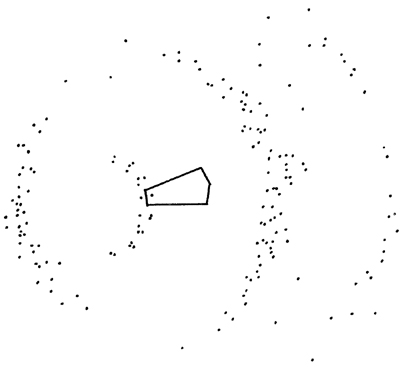
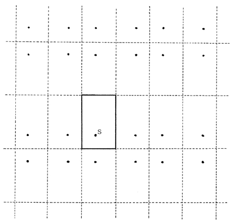
Having made this program, we are now in a position to use it to gain some insight into how reverberation works. The first case we will discuss, however, is the classical example that needs no program : the rectangular room. This is one case where so many of the phantom sources fall on top of each other that they form a rectangular array, as is shown in figure 10. This is similar to the barbershop mirror phenomenon, where one sees an endless array of phantom sources streaching off to infinity in both directions, some facing forward and some facing backward. The point of discussing this case, however, is to show that no artificial reverberator based on recirculating delays can ever be identical to even this geometrically simple case. This is immediately clear from putting a listener into the room. The contributions from just the row that crosses the room are at distances that are related by the square root of the sum of the squares of the vertical and horizontal distances. Granted that the vertical distance increases in regular increments of multiples of the room hight, the resulting distances are not integer multiples of anything. In the limit as the sources get further and further away, the distances become almost equally spaced, implying that although the early response could never be simulated exactly by recirculating delays, it may be possible to approximate the late response. This also gives us some insight as to why typical artificial reverberation is always easily distinguishable from natural reverberation.
Following an idea reported by Schroeder (1970), we may simulate directly the early response by a finite impulse response filter, and simulate the late response with a standard reverberator, as is shown in figure 3. Here we choose to simulate the first n delays separately with separate gains, then to send the delayed signal into a standard reverberator, R(z), with its own gain of g. We must then ask what are the design requirements of this reverberator and how do they differ from stand-alone reverberators. Our experience is, sadly enough, that they do not differ from stand-alone reverberators, in that they need all the usual complexity. Again, the most pleasing and natural sounding system we have tried is the comb-all-pass combination with 6 comb filters, with low-pass in the feedback loops, and 1 all-pass. It is not necessary, however, to use the very long delays (for instance, the 10 to 15 millisecond range). All the design guides described in previous sections apply for these reverberators, including considerations of total reverberation time, ratio of minimum delay to maximum, etc. etc.
Figure 10
Phantom source patterns for a rectangular room form perfectly regular patterns of rows and columns. Any room shape which tesselates a surface by reflecting across each of its edges will have such a repeating pattern of sources. Such figures include equilateral triangles, for instance, and regular hexagons.
The basis of the rational for simulating just the early echos is the various perceptual phenomena that ensue with the spacing of echos. With the case of two impulses spaced closely in time, the separation of these two impulses determines a wide range of perceptual effects. Certainly if the two pulses are more than 30 to 50 milliseconds apart, they will be heard as two separate and distinct pulses. Between this figure and 1 or 2 milliseconds, they will not be heard as distinct pulses, but the timbre of the combination will change (Green 1971). At less than 1 millisecond separation, the timbre of the ensemble does not change any further, but if presented binaurally, still give rise to localization effects down to a spacing of tens of microseconds. With this in mind, it is clear that if we simulate the discrete echos down to a limit of 1 millisecond before switching to a recirculating delay reverberator, we can capture much of the effect of a specific concert hall, except possibly for localization effects.
Before we leave the topic of computer simulation of geometric acoustics, we should mention at least two other interesting results of these simulations. First of all, one might criticize the approach for being 2-dimensional. However, the formulas do not get terribly more complex when 3-dimensional geometry is used, so one could write the simulation program entirely in 3 dimensions. The winged-edge polyhedra model of Baumgart (1972, 1974, 1974, 1975) seems almost ideally suited to this in that the faces are canonically ordered, making inside/outside determination simple, and that local connectedness is simply represented. Our results seem to imply that in many cases this is not necessary. With many of the rectangular concert halls, such as the Boston Symphone Hall, the problem can be approximated by two 2-dimensional problems : one in the vertical plane and one in the medial plane. A 3-dimensional path would imply a sort of helical path which is somewhat uncommon in rectangular halls.
Another interesting result is that non-parallel walls do not necessarily imply uniform echo patterns. Figure 8b, for instance, shows a simulated hall with non-parallel walls that exhibits a highly regular impulse response, regardless of source placement. The phantom sources cluster in circles about the source of radii roughly twice the length of the hall. Likewise, the fact that the best-liked concert halls are exactly rectangular in shape (Vienna Grosser Musikveriensaal, Boston Symphony Hall, Amsterdam Concertgebouw) leads one to wonder indeed if parallel walls really do have anything to do with the subjective characteristics of the halls. It would seem that the detailed structure and composition of the walls are more perceptually important than the overall shape.
We have described several different approaches to simulating concert hall reverberation. One approach is largely disconnected from physical reality in the use of recirculating delays to simulate the echo patterns of concert halls. The other approach is a computer simulation of the actual reflection pattern of a concert hall based upon its geometry.
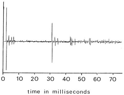
The only problem with simulating room reverberation in this way, that is with direct geometrical simulation of the room acoustics, is that it doesn't sound at all like real rooms. This somewhat startling fact means that one or more of our assumptions does not hold water. To follow this up further, we obtained copies of the responses of many natural concert halls which were taken by Schroeder, et al (1974) and Gottlob (1975). Careful examination of these impulse responses made it quite clear that a very important consideration that we have been ignoring is the effect of diffusion. This comes about when walls are not in fact flat but are irregular. This is, of course, true in all respected concert halls. Our own Boston Symphony Hall has fluted side walls and box well ceiling, each of which furnishes a plethora of new phantom sources. Figure 11 shows the doublet response of the old New York Philharmonic hall before reconstruction, obtained by placing a powerful spark gap device on stage and an omnidirectional microphone in a particular seat in the audience. We notice immediately that some distinct echos are visible, but a great confusion soon follows with virtually no silent portions. This confusion is clearly the result of the infinite multiplicity of diffused sources caused by every little irregularity in the hall. We can, of course, convolve our music directly with this response (corrected for the spectrum of the spark gap itself) to produce the sound of that concert hall, but with even a 25 KHz sampling rate and a 2.0 second reverberation time, this comes out to 50,000 multiplications and additions per output sample. This is clearly only in the domain of very patient researchers with great quantities of computer time available. Even with fast Fourier transform techniques (Stockham 1966), we consumed about 6 minutes of computer time (PDP-10) for every second of sound time thus processed. We might then ask if there is any way that we can simulate at least some of these effects without such an obese expenditure of computer time. Indeed, it would appear that a modification of the Schroeder design of figure 3 can give somewhat improved results at only a moderate increase in computation time.
Figure 11
Doublet response (echogram) of the New York Philharmonic Hall before reconstruction. This response was collected by D. Gottlob, et all (1974). Note that even though certain distance reflections are clear, there is a great deal of activity throughout the response.
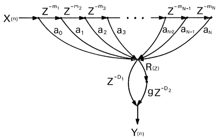
Figure 12 shows our new formulation. As before, we have N delays which simulate the first N reflections plus the direct signal. This presumably takes care of the first 40 to 80 milliseconds of the decay. This entire signal is now forwarded to the reverberator, R(z), which is then added into the early decay with a gain of g. What this provides is that all the density of the first N reflections is then repeated many many times by the recirculating delays of the reverberator. The delays D1 and D2 are set such that the first echo from the reverberator coincides with the end of the last echo from the early response. This means that either D1 or D2 will be zero, depending on whether the total delay of the early echo is longer or shorter than the shortest delay in the reverberator.
Adding this separate discrete early echo makes a substantial difference in the sound, and in fact, if the actual room response is used for the early delays, the sound does begin to approach the sound of the real concert hall. Since using the first 80 milliseconds of the actual room impulse response is still well beyond the bounds of sanity, except in certain restricted circumstances for research purposes, we may then ask how simple can this early response be and still give a rich, life-like sound.
Various ways were tried to synthesize a suitable early response from using the results of the geometric simulation of a room, real or fictitious, to choosing random numbers to determine the positions and amplitudes. Many problems became clear while attempting to do this. It would seem that one cannot just compute a bunch of impulses at random and expect it to sound good, in that there is always the possibility that it will form a very strong comb filter effect. Even if the positions are chosen to be prime numbers of samples from the origin, the differences among them in time may well be highly composite. This is easy to see when one realises that the sum or difference of two prime numbers is always divisible by two. As a result, we can not give at this time any general method for finding different early responses that will sound good. We have, essentially by trial and error, determined at least two that sound reasonable without too much coloration of the sound. These are given in table ITT. There is a 7-tap section and a 19-tap section. The first tap is the direct signal and it can be changed to provide more or less reverberation if desired.
Figure 12
Signal flow diagram of reverberator using FIR portion to simulate early echos and an IIR portion, denoted by R(z) above, to simulate the late portion. Delays D1 and D2 are adjusted so that the last pulse from the FIR section corresponds roughly in time with the first pulse to exit from the IIR section. One or the other of D1 and D2 will be zero for any given diagram.
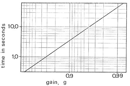
Thus, we are now in a position to give a systematic technique for designing a reasonably good sounding reverberator, albeit not one that corresponds to any particular concert hall in existance today. The formulation of figure 12 with the 19-tap model is preferred, although the 7-tap section can be used, or even a no tap system is computer time is at a premium. The recirculating part, as mentioned before, should consist of 6 combs in parallel, each with a first order lowpass filter in the loop. The outputs of the 6 combs should be summed and forwarded to a single all-pass network with a gain of 0.7 and a delay of about 6 milliseconds. The gains of the low-pass filters in the feedback loops of the combs should be set to the values from figure 6 for the delay used. The delays should be linearly distributed over a ratio of 1:1.5 with the shortest delay being about 50 milliseconds. Again, if computer memory is at a premium, this can be reduced to as low as 10 milliseconds without gross degradation. The delay lengths in samples should be set to the closest prime numbers to prevent exactly overlapping pulses, although with higher values of g1 in the feedback filters, the sensitivity to the exact length of the delay becomes negligable. The gains, g2, of each comb should be set to g(1 - g1) where now determines the overall reverberation time. Figure 13 shows the relation between total reverb time as a function of computed at a sampllng rate of 25 KHz. We originally computed the reverb time both as twice the time to fall from, 5 to 35 dB, and as the time to fall from 0 to 60 dB, but these numbers were quite similar (within 10%) at most values of g except very small or very large ones. The reverb time of this system can be estimated without use of figure 13 as .366/(1 - g) to an error to about 10%. Likewise, the gain can be computed for a given value of reverberation time as 1 - .366/T where T is the desired reverberation time in seconds. Note that this will change with sampling rate, but the deviation should not be too drastic. Likewise, this time will scale directly with the delay lengths, as long as the 1:1.5 ratio is maintained between the shortest comb delay and the longest.
Figure 13
Reverberation time of the 6-comb, 1-allpass reverberator assuming that the low-pass filter gain, g1, is set according to the guides of figure 6 and the delays are set according to table II. In this case, the gain, g, will determine the reverb time. This curve can be approximated by the function .366/(1 - g). Conversely, g can be estimated as 1 - .366/T where T is the reverberation time desired (in seconds)
In the course of this work, it became quite clear that all the geometric simulations of concert hall acoustics that have been done to date result in a simulated room reverberation that does not sound at all like real rooms. This is probably due to the effect of diffusion of echos due to irregularities in the reflecting surfaces and the fact that the spectrum of the echo is modified by the reflection in a manner that depends strongly on the angle of incidence.
Despite these facts, we have been able to achieve a good sounding, smooth artificial reverberation system that regardless of the fact that it does not sound like actual concert halls, does sound good enough to be used everywhere that artificial reverberation is desired, and does eliminate some of the problems that plagued earlier reverberation schemes, such as "fluttery" response to short, impulsive sounds and metallic sounding decay. We also found a much larger number of non-useful new unit generators than useful new unit generators.
There are several topics that were revealed in the course of this study that would make excellent material for further study, and excellent doctoral dissertation topics. These might include the foIIowing :
As usual, it would be out of the question to attempt to thank individually all the people and institutions that went into this research. My thanks, as always, go to my dear collegues at Stanford : J. Chowning, J. Grey, G. Loy, L. Rush, and P. Wood. Thanks to D. Gottlob who so patiently sat through two harrowing days of digitizing all these impulse responses with us at IRCAM. Thanks also to Jean Derochapt, my co-conspirator and programming aid in this work, who got my imagination going on this subject. Finally, of course, to the Institut de Recherche et Coordination Acoustique/Musique (commonly known as IRCAM) for providing one of the few places in the world where this kind of in-depth research can be done, and to my boss, Gerald Bennett, for letting me heed my notions in plowing through the maze of half-baked ideas.
Table IIITap times (in seconds) and gains for a reasonable-sounding 7-tap FIR section for reverberation. Tap number corresponds to the subscript of the coefficient (ai) and delay (mi) shown in figure 12.
TAP TIME GAIN 0 0 1.00 1 .0199 1.02 2 .0354 .818 3 .0389 .635 4 .0414 .719 5 .0699 .267 6 .0796 .242 Tap times (in seconds) and gains for a reasonable-sounding 19-tap FIR section for reverberation. These were taken from a highly idealized geometric simulation of the Boston Symphony Hall.
TAP TIME GAIN 0 0 1.0 1 .0043 .841 2 .0215 .504 3 .0225 .491 4 .0268 .379 5 .0270 .380 6 .0298 .346 7 .0458 .289 8 .0485 .272 9 .0572 .192 10 .0587 .193 11 .0595 .217 12 .0612 .181 13 .0707 .180 14 .0708 .181 15 .0726 .176 16 .0741 .142 17 .0753 .167 18 .0797 .134
____________________________
Server © IRCAM-CGP, 1996-2008 - file updated on .
____________________________
Serveur © IRCAM-CGP, 1996-2008 - document mis à jour le .