Tous droits réservés pour tous pays. All rights reserved.
| Serveur © IRCAM - CENTRE POMPIDOU 1996-2005. Tous droits réservés pour tous pays. All rights reserved. |
TFTS'97 (IEEE Time-Frequency and Time-Scale Workshop 97), Coventry, Grande Bretagne, août 1997
Copyright © IEEE 1997
In consequence, it is not surprising that additive analysis and synthesis of musical signals have recently received a great deal of attention. Even though the, now classical, additive sinusoidal analysis is based on rather simple principles, it has been very successful. The first goal of this paper is to examine this method, the reasons of its success and its weaknesses. The second goal is to try to extrapolate from our conclusions in order to propose new reasearch directions for musical signals analysis.
In section 2, we present additive sinusoidal analysis. The main drawbacks of the classical method are then explained in section 3 and some important improvements are briefly exposed. In section 4 we try to understand the advantages of additive analysis as well as its limitations. In section 5, under the term Elementary Waveforms, we present some new directions better suited for the analysis of musical sound signals.
With ai (t)
 0 the amplitude and
  i(t) the
phase of the sinusoidal partial:
i(t) the
phase of the sinusoidal partial:
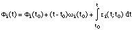
ci (t)=ai (t)cos(A first important assumption underlying (often implicitly) sinusoidal models is that ci (t) locally ressembles a pure sinusoid. This means that a(t) should be a slowly varying signal, i.e. a low pass signal with a bandwith Ba and that
i(t) is locally linear in t up
to a small correction term. If locally around t0 is defined
as t [t0-
[t0- , t0+]:
That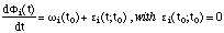
 i is small can be stated more precisely by
saying that
i is small can be stated more precisely by
saying that  i(t) is a slowly varying signal, i.e. a low pass
signal or that cos(i(t)) is approximately a band limited signal
for t[t0-, t0+], with a
bandwith Bf around i(t0). However, we
will see in section 3 that the first assumption presented here above is only a
rough approximation. In particular, the frequency behavior should not be
formulated in terms of local variations of relative value but in
terms of local variations of relative slope. Similarly, amplitude
behavior should allow some fast variations such as is found in the attacks of
percussive sounds.
i(t) is a slowly varying signal, i.e. a low pass
signal or that cos(i(t)) is approximately a band limited signal
for t[t0-, t0+], with a
bandwith Bf around i(t0). However, we
will see in section 3 that the first assumption presented here above is only a
rough approximation. In particular, the frequency behavior should not be
formulated in terms of local variations of relative value but in
terms of local variations of relative slope. Similarly, amplitude
behavior should allow some fast variations such as is found in the attacks of
percussive sounds.Speech and musical sounds always have random components, often heard as a noise superposed for instance on the harmonic part. A second assumption often underlying a sinusoidal model is that the number I of sinusoidal partials is limited. Therefore, a purely sinusoidal model with slowly varying parameters can hardly represent all of a real signal x(t) and needs to be completed with a non-sinusoidal residual part r(t):
r(t) = x(t) - s(t)Another argument in favor of a non-sinusoidal residual part r(t) is that the residual should be considered as a random signal in case of transformations such as time compression or expansion. In consequence, classical representations of random signals are better suited for the residual. It is common to represent only the short-time magnitude frequency content of the residual by a spectral envelope G(t,
) [Serra 89]. If n(t) is a white
gaussian noise and G(t,) is the Fourier Transform of a time-varying
impulse response g([theta],t), then the model of the residual is:
This filtering can be implemented in the time domain or in the frequency domain. If R(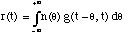
,t) and N(,t) are the Short-Time Fourier
Transforms of r(t) and n(t) respectively, then:
Fig. 1. Peaks found in successive analysis frames are grouped into tracks,i.e. sinusoidal partials.
Let x[n] be the analysed discrete signal, h[n] the analysis window and
X(n,k) its STFT at time n and frequency
k:
Since we look at the STFT of a given frame around time n, let us drop index n and write X(, (1)
k)=X(n,k) A peak of the
magnitude of the STFT obtained by Discrete Fourier Transform of size N,
|X(k)|, is found at index  when
when
|X(A peak at index
supposedly indicates the presence of a
sinusoidal partial at a near-by frequency  (
(  ). The frequency i(t) and
the amplitude ai(t) of this sinusoidal partial can be considered
constant around time m, with values and A respectively. Henceforth, the
shape of|X(k)| around index is the sampled shape of
|H(-)|, i.e. of the Fourier Transform of h[n] translated at the
frequency . To estimate and A, since h[n] is usually a symmetric
window, one can use the second order approximation of H(-) around
which is given by a quadratic function centered on . This is why
a quadratic approximation of |X(k)|, in the neighborhood of
index , is performed [McIntyre 92]. Then the center and the maximum
amplitude of this function are taken as an estimation of and A
repectively. Similarly, the local phase of the sinusoidal partial is
obtained as a weighted average of the phase of X(k) in the
neighborhood of index . The role of the weighting factor is to increase
the importance of high amplitude values |X(k)| in order to
diminish the effect of relatively low amplitude noise superposed on the
sinusoidal partial.
). The frequency i(t) and
the amplitude ai(t) of this sinusoidal partial can be considered
constant around time m, with values and A respectively. Henceforth, the
shape of|X(k)| around index is the sampled shape of
|H(-)|, i.e. of the Fourier Transform of h[n] translated at the
frequency . To estimate and A, since h[n] is usually a symmetric
window, one can use the second order approximation of H(-) around
which is given by a quadratic function centered on . This is why
a quadratic approximation of |X(k)|, in the neighborhood of
index , is performed [McIntyre 92]. Then the center and the maximum
amplitude of this function are taken as an estimation of and A
repectively. Similarly, the local phase of the sinusoidal partial is
obtained as a weighted average of the phase of X(k) in the
neighborhood of index . The role of the weighting factor is to increase
the importance of high amplitude values |X(k)| in order to
diminish the effect of relatively low amplitude noise superposed on the
sinusoidal partial.The relatively simple detection and estimation procedure described here above has weaknesses which are detailed in section 3. However, it should be underlined that it has known a great success because it is fast and very robust. It can deal with the hundreds of sinusoidal partials encountered in musical signals and does not suffer from model-order determination and numerical or computational limitations which are common, for example, in parametric methods [Laroche & Rodet 89b], [Laroche 93a].
The second step of sinusoidal parameter estimation is the grouping of successive analysis frame peaks into tracks. This tracking is usually based on a heuristic approach [McAulay & Quatieri 86], [Serra 89] which matches peaks in successive frames while allowing deaths and births of tracks. It simply grows trajectories, iteratively frame after frame, in the direction of increasing time: for each frame successively, the tracks which still appear in the current frame are possibly continued provided there is a convenient peak in the next frame according to an optimal frequency match. When needed, some tracks are terminated and new tracks arise. We will not detail this algorithm here since we prefer a well grounded statistical approach presented in section 3.4.
Estimation of the spectral envelope of the residual signal around time t,
G(,t), can be done with any usual AR estimation technique [Kay 88]. Such
a technique provides the P coefficients ap(t) of an all-pole filter
with magnitude transfer function G(,t). The coefficients
ap(t) are well suited for time-domain filtering of a noise n(t) at
the synthesis stage. In practice, the ap(t) are only estimated
around successive times tl ,l=1, 2, 3,..., with a step
tl+1-tl on the order of 5 to 20 milliseconds. Cepstral
estimation can also be used on sliding window STFT R(,t) of r(t).
Cepstral estimation provides P cepstral coefficients cp(t) which are
well suited for frequency domain filtering of a noise n(t) at the synthesis
stage. When estimating the spectral envelope G(,t), a nonlinear
frequency scale, such as the Mel or the Bark scale, is appealing
since is reflects some properties of human perception. Some authors [Serra 89],
[Goodwin 96] have proposed to simply represent the magnitude short-time
spectrum |R(,t)| by its mean value in channels distributed on such a
nonlinear scale. This representation also is well suited for frequency domain
filtering at the synthesis stage, since it requires only a mutiplication of the
STFT of the noise n(t) by |R(,t)|.
k). Let us again drop index n and write
X(k)=X(n,k). If H() is the Fourier
Transform of the analysis window h[n], this problem can be viewed as the
detection of the presence of a scaled and sampled version of the signal
H() in the signal X(k). Therefore, it is
natural to look for the maxima of the cross-correlation function  of H
and X. If W is the bandwith of the low-pass signal h[n], then H() can be
considered as negligible outside the interval [-W,W] and the computation of
() is simplified:
of H
and X. If W is the bandwith of the low-pass signal h[n], then H() can be
considered as negligible outside the interval [-W,W] and the computation of
() is simplified:
Each maximum |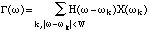
()| indicates a sinusoidal partial
candidate at frequency . An estimation of the amplitude A and
of the phase of the partial can then be derived. Defining at a
norm for H and X by:
and
we obtain:
Note that this computation also provides a measure v
of the likeness between the observed peak and the peak which would result
from a pure steady sinusoid (in which case v=1):
A sinusoidal likeness measure (SLM) v
<1 indicates
the presence of noise or of other sinusoidal components in the neighborhood of
, or that the detected sinusoidal partial has fast varying parameters.
The third case, fast variation, is examined in section 3.3 and 3.5. The second
case, close-frequency partials, has been looked at by [Maher & Beauchamp
94]. If one can disregard the two last cases, then the SLM v
is similar to the so called voicing index of speech signals. But the SLM
v(n) is here a function of two variables, the analysis time n
and the frequency . Errors on the speech voicing index at time n have
serious consequences for speech coding or synthesis. On the other hand, errors
on the SLM v(n) for some are of little consequence
and are statistically compensated for by other v values. This
SLM function v(n) has been very successfully used for speech
coding or synthesis [Griffin & Lim 85], [Rodet & al. 87] as well as for
musical sound analysis and synthesis [Rodet & al. 88], [Doval 94].
In [Laroche 89a] a time-domain method is developped to estimate complex amplitudes (i. e. real amplitudes and phase deviations), when mean frequency values are known. Note that phase deviation is then equivallent to frequency variation. The model of the complex amplitude of the ith sinusoidal partial is a low order (e.g. 3) polynomial of time n:
The model
 [n] of the signal is a sum of I sinusoidal partials. With
zi=exp(ji):
[n] of the signal is a sum of I sinusoidal partials. With
zi=exp(ji):
Let, (2)
be the column vector
=([1],[2],...,[N])t where N is the analysis
frame length, bi=(bi,0,bi,1,
...bi,q)t,
B=(b1|b2|...|bI)t
and
 =[1|2|...|I|]
where
=[1|2|...|I|]
where
Then we can write equation (2):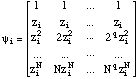
Minimisation of
leads to:
B=[The method has been applied successfully by [Laroche 89a] to find the amplitude and phase variations of sinusoidal partials of percussive sound signals, after the mean frequencies were found by Prony's method. This simultaneous determination of amplitude and frequency variations would be a useful complement of the classical sinusoidal analysis where mean frequency values are estimated on spectral peaks.
Naturally, sinusoidal partial parameter evolution also appears in the STFT,
leading to a distorsion of peaks from the pure-sinusoid peak shape as
mentionned in section 3.1. The distorsion caused by linear frequency modulation
(LFM) and exponential amplitude modulation (EAM), in a given STFT
X(k)=X(n,k), is examined in [Masri 96]. In
the case of a pure sinusoid, the phase of the FFT bins,
Arg{X(k)}, in the vicinity of the corresponding peak, is
constant. In the case of modulation, this phase shows a variation
 (r) which is a function of the frequency
r relative to the peak center. Experimental measures show
that LFM, up to 16 bins of modulation per frame, causes a variation
f(r) which is increasing with
r for small |r|. Similarly, EAM, up to 6 dB
of modulation per frame, causes a variation
a(r) which is proportional to
r for small |r|. Therefore, when only one
type of modulation appears and is not too large, it can be estimated from the
phase spectrum. Furthermore, for small |r|, the phase
variations due to LFM and EAM are additive. But, since
f(r) has even symmetry and
a(r) has odd symmetry, their cumulative
effect produces a global variation
f(r)+a(r)
with distinctive shapes according to the slope signs of
f(r) and
a(r). Therefore, simultaneous LFM and EAM
can be estimated from the phase spectrum. The method has been successfully
applied on simulated audio signals. However, for real musical signals, where
additive interference from the more prominent peaks affects the phase profile
accross less prominent neighbouring peaks, the described implementation is not
resilient enough [Masri 96]. But it seems that the extracted slope information
could be profitable at the partial tracking stage.
(r) which is a function of the frequency
r relative to the peak center. Experimental measures show
that LFM, up to 16 bins of modulation per frame, causes a variation
f(r) which is increasing with
r for small |r|. Similarly, EAM, up to 6 dB
of modulation per frame, causes a variation
a(r) which is proportional to
r for small |r|. Therefore, when only one
type of modulation appears and is not too large, it can be estimated from the
phase spectrum. Furthermore, for small |r|, the phase
variations due to LFM and EAM are additive. But, since
f(r) has even symmetry and
a(r) has odd symmetry, their cumulative
effect produces a global variation
f(r)+a(r)
with distinctive shapes according to the slope signs of
f(r) and
a(r). Therefore, simultaneous LFM and EAM
can be estimated from the phase spectrum. The method has been successfully
applied on simulated audio signals. However, for real musical signals, where
additive interference from the more prominent peaks affects the phase profile
accross less prominent neighbouring peaks, the described implementation is not
resilient enough [Masri 96]. But it seems that the extracted slope information
could be profitable at the partial tracking stage.
k)|
of the signal x[n], as given by equation (1). In this equation, h[n] is a
classical window, such as the Hamming window. The computation is done with a
Discrete Fourier Transform [Rabiner & Schafer 78] and the
k, k=1, 2, ... K, are regularly spaced frequencies. Since we
consider the STFT for a given n, let us simply write
X(k)=X(n,k). When two sinusoidal partials
have nearby frequencies separated by  f Hertz, in order that
|X(k)| exhibit two peaks, it is necessary that the window
length L is large enough:
f Hertz, in order that
|X(k)| exhibit two peaks, it is necessary that the window
length L is large enough:L > q/where L is in seconds, q depends on the window main lobe width and is on the order of 3.5. Let us take for example a harmonic sound with a fundamental frequency of 110 Hz (which is heard as the note A2). Its sinusoidal partials are 110 Hz apart and L should be greater than 3.5/110, i.e. 32 ms. In polyphonic sound signals, partials can be even much closer and the length L should be accordingly larger. Note that the minimum frequency distance between sinusoidal partials is often unknown. A large window is a great inconvenience when sinusoidal parameters vary substantially over a time segment L. In particular, fast transitions such as consonnants or percussive attacks are smoothed. The problem is even worse for sinusoidal partials the frequency of which varies substantially. As an example, if the fundamental frequency varies by d Hertz on the window length L, then the ith partial varies of id When i is large, this important frequency modulation induces such a spreading of their spectrum that correponding peaks are smeared in |X(
k)| and their detection fails. Another weakness of the
standard sinusoidal analysis is that it does not take into account the
influence of sinusoidal partials close in frequency which slightly alter the
estimation of frequency and amplitude of a given sinusoidal partial.f.Let us still write
X(k)=X(n,k) for the STFT of the
signal at time n. The model of the signal is based on the assumption of a
sum of sinusoidal partials with amplitude and frequency constant over the
window duration L, ai=ai[n] and
i=i[n] and a local phase
 i:
i:
Therefore, the model of the Fourier Transform is: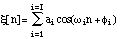
where H(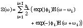
) is the Fourier Transform of the analysis window h(n).
The method consists in identifying the parameters for which the model best fits
the observation X(k) according to a least squares criterion.
The identification is realised by an iterative algorithm which alternatively
improves the estimates of amplitudes using the previous estimates of
frequencies and improves the estimates of frequencies using the previous
estimates of amplitudes [Depalle & Hélie 97]. Initial estimates are
obtained from the standard sinusoidal analysis using a relatively long window
with a small bandwidth (e. g. a rectangular window). At each iteration, the
amplitude optimisation is a simple linear problem. Since the frequency
estimation problem is nonlinear, a simple linear optimisation is performed at
each iteration: the equation is linearised around the vector
{i-k, k=1, 2, ... K} in order to lead to a
linear problem. One difficulty is that the algorithm can then converge, not to
the main-lobe maximum, but to a secondary maximum corresponding to a sidelobe.
In order to avoid that, Depalle and Hélie [Depalle & Hélie
97] have designed and used a new family of analysis windows without sidelobes.
Other improvements of the algorithm are given in the above two references. This
algorithm is shown to converge rapidly to the correct parameter values even
when it is initialized with rather poor approximations. It also remains
efficient at low signal-to-noise ratios (e.g. 10 power dB).
On the contrary, the procedure described in [Depalle & al. 93a], [Depalle & al. 93b], copes with these problems by globally optimizing the set of tracks. The peak tracking problem is formulated in terms of a Hidden Markov Model (HMM) [Rabiner 86]. The optimization is performed in a given time interval T according to a statistical criterion of slope continuity for all the sinusoidal parameters. Therefore, the optimal set of trajectories is found as the highest probability state sequence, by means of the Viterbi algorithm [Rabiner 86]. Note that the use of parameter slopes rather than parameter values, while being consistant with the first assumption of a sinusoidal model (see section 2.1), enables one to track time-varying partials as easily as constant ones, and solves the problem of detecting crossing trajectories.
We shall only indicate here a few features of the algorithm. Since the number
of tracks can be in the hundreds, the biggest problem is to reduce
computational complexity. Therefore, the Viterbi algorithm is applied on a
window length of T frames, which slides frame by frame, and some constraints on
index combinations, maximum number of tracks, etc., are added. Furthermore, the
algorithm considers only the possible combinations of peaks between successive
frames. Sinusoidal parameters are used to compute state transition
probabilities [Depalle & al. 93] which favour slope continuity and disfavour spurious peaks. At time m, there are hm peaks Pm[i], 1 < i  hm. Each track is labelled by an
index greater than zero. The problem is to associate an index Dm[i],
1 < i hm, to each peak Pm[i]. When a
peak Pm[i] is considered as a spurious one, it is associated with a
null index Dm[i] = 0. A state Sm is defined by an ordered
pair of vectors (Dm-1, Dm) and the observation is defined
by an ordered pair of integers (hm-1, hm). The optimal
sequence of states Sm=(Dm-1, Dm) is found by
means of the Viterbi algorithm, which maximises the joint probability of state
and observation sequences leading to a globally optimal solution. Then the
tracks are defined by the sequence of vectors Dm from the state
sequence.
hm. Each track is labelled by an
index greater than zero. The problem is to associate an index Dm[i],
1 < i hm, to each peak Pm[i]. When a
peak Pm[i] is considered as a spurious one, it is associated with a
null index Dm[i] = 0. A state Sm is defined by an ordered
pair of vectors (Dm-1, Dm) and the observation is defined
by an ordered pair of integers (hm-1, hm). The optimal
sequence of states Sm=(Dm-1, Dm) is found by
means of the Viterbi algorithm, which maximises the joint probability of state
and observation sequences leading to a globally optimal solution. Then the
tracks are defined by the sequence of vectors Dm from the state
sequence.
This algorithm has been implemented at IRCAM by G. Garcia. Other computational cost reductions have been applied. In particular, the Viterbi algorithm has been replaced by a more efficient one taking advantage of the factorised structure of transition probabilities and eliminating computational redundancy. IRCAM's HMM tracking algorithm has been successfully used for sound analysis, processing and synthesis for research and for musical creation. As an example, it is possible to analyse polyphonic music comprising simultaneously several instruments, chords and percussion sounds. Examples will be played at the conference.
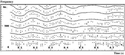
However, there are sound signals for which sinusoidal analysis does not seem so well adapted, typically signals where excitation departs from periodicity. Curiously enough, sinusoidal analysis is also used for speech signals even though they often fall in the last category. The classical model of glottal speech production [Fant 70] consists of short pulses filtered through the vocal tract. Firstly, variations of vocal tract transfer function can be appreciable at the time scale of three glottal periods. Secondly, time locations of pulses can be far from periodical. We already noted in section 3.3 that high rank partials cause difficulties even for small fundamental variations. Figure 2 shows another case, i.e. a speech waveform resulting from irregular pulses, as often occurs at the end of a sentence (it is sometimes called vocal fry). Sinusoids make sens when, in a given frequency band, a waveform repeats periodically at least three times. On the contrary, signals like the one in figure 2 suggest the use of other methods based on waveforms better localised in time when needed, sometimes called Elementary Waveforms (see section 5).
Finally, the standard noise source and filter model represents non-sinusoidal and random components in a very unsatisfactory way [Goodwin 96]. Moreover, the fact that two totally different analysis techniques are needed is a weakness which leads to difficulties since the separation of sinusoidal and random components is not based on any solid grounding.
Figure 2. A speech waveform resulting from irregular pulses, as often occurs at the end of a sentence.
In [Liénard 87], a narrow band-pass filter bank is used to ensure locality in frequency. The signal at the output of each filter is segmented at successive minima of its amplitude envelope. Each segment is considered as an EW. The method has been used for speech analysis and synthesis.
Note that sinusoidal analysis starts with a STFT at arbitrary regularly spaced times, then look for specific peak patterns in the STFT. On the other hand, some EW analyses start with arbitrary regularly spaced band-pass filtering, then look for specific patterns in filter outputs. Matching Pursuit, presented here below, does not favour time or frequency but, at each step, looks for a time and a frequency elementary waveform position, as well as a scale, which are optimal according to the properties of the signal under analysis.
Pursuit algorithms, such as Matching Pursuit (MP) [Mallat & Zhang 93] or
Basis Pursuit [Chen & Donoho 95] have been designed to overcome these
difficulties. The decomposition vectors are selected among a redundant
family, called a dictionary, of EWs well localised in frequency and
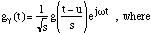
time. In MP, the EWs which constitute the dictionary have three parameters, a
scale factor s, a time position u and a modulation frequency (note
that, unlike in Wavelets, scale and frequency are independant). With
 =(s,u,):
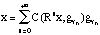
is a Gaussian fonction with unit norm. A MP is an iterative algorithm which decomposes a signal x over dictionary vectors as follows. Let us write Rnx a residue at step n, starting from R0x=x. At each step, the vector selected in the dictionary is the one which matches Rnx at best, i.e. such that: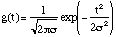
where,
is the set of all possible values for and
C(x,g) is a correlation function which measures the
similarity between x and g. The residue for the next step is
then:
Finally, the signal is represented as: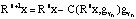
In [Mallat & Zhang 93], the correlation function C is the inner product C(x,g
)=<x,g>. This
decomposition is relatively fast to compute, gives a good resynthesis with a
limited number of vectors and exhibits the different structures of the signal
at different scales [Gribonval & al. 96a], [Gribonval & al. 96b].
However, these references show that the chosen correlation function C leads to
inadequate representations of some structures, such as a sinusoid the envelope
of which varies rapidly. Therefore, a High Resolution MP (HRMP) algorithm is
introduced. It uses a different correlation function which allows the pursuit
to emphasize local fit over global fit at each step. HRMP performs a better
time-resolution than MP so that, in audio applications, attack-patterns
recognition or processing is improved.
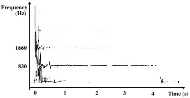
Fig. 3. Time-frequency distribution of a G5 sharp piano note, obtained with HRMP
The time-frequency distribution of a G5 sharp piano note, obtained with HRMP, is displayed in figure 3. One can easily distinguish long horizontal lines due to large-scale vectors well defined in frequency around 830 Hz, 1660 Hz, etc.. They correspond to the damped sinusoidal quasi-harmonic modes of the string. On the contrary, vertical lines corresponding to small-scale transient structures are visible at the attack and at the release of the damper of the piano. This example shows how HMRP provides a time-frequency representation adapted to the specificities of sound signals. The elements of this representation are easily related to perceptually important structures such as fast transients, or sustained sinusoidal partials.
[Chen & Donoho 95]S. Chen, D. L. Donoho, Atomic decomposition bt basis pursuit, Technical report, Statistics Department, Stanford University, 1995.
[Coifman & Wickerhauser 92]R Coifman, M.V. Wickerhauser, Entropy based algorithms for best basis selection, IEEE Trans. Inform. Theory, 38 (2):713-718, P&rch 1992.
[Corrington 70] M. S. Corrington, Variation of Bandwidth with Modulation Index in Frequency Modulation, Selected Papers on Frequency Modulation, edited by Klapper, Dover, 1970 [Depalle 93a] Ph. Depalle, G. García, X. Rodet. Tracking of partials for additive sound synthesis using hidden Markov models. IEEE ICASSP-93 , Minneapolis, Minnesota, Apr. 1993.
[Depalle 93b] Ph. Depalle, G. García, X. Rodet. Analysis of Sound for Additive Synthesis: Tracking of Partials Using Hidden Markov Models, Proceedings of International Computer Music Conference (ICMC'93),Oct. 1993.
[Depalle & Tromp 96] Ph. Depalle, L. Tromp, An improved additive analysis method using parametric modelling of the short-time Fourier transform, Proceedings of International Computer Music Conference (ICMC'96), Clear Water Bay, Hong-Kong, August 1996.
[Doval & Rodet 93] B. Doval, X. Rodet, Fundamental Frequency Estimation and Tracking using Maximum Likelihodd Harmonic Matching and HMM's Proc. IEEE- ICASSP 93, pp. 221-224.
[Doval 94] B. Doval, Estimation de la Fréquence Fondamentale des signaux sonores, PhD. Thesis, Université Paris-6, Paris, 1994.
[Fant 70] G. Fant, Acoustic Theory of Speech Production, Mouton, 1970.
[Fitz & al. 95] K. Fitz, L. Haken, B. Holloway, Lemur - A Tool for Timbre Manipulation, Proc. Int. Comp. Music 1995, Banff, Sept. 1995.
[George & Smith 92] E. B. George, J. T Smith, Analysis-by-Synthesis/Overlapp-Add Sinusoidal Modeling Applied to the Analysis and Synthesis of Musical Tones, J; Audio. Eng. Soc., Vol. 40, No. 6, June 1992.
[Goodwin 96] M. Goodwin, Residual modeling in music analysis-synthesis, Proc IEEE-ICASSP, Atlanta, GA, pp. 1005-1008, May 1996.
[Gribonval & al. 96a] R. Gribonval, E. Bacry, S. Mallat, Ph. Depalle, X. Rodet, Analysis of sound signal with high resolution matching pursuit, Proceedings of the IEEE Conference on Time-Frequency and Time-Scale Analysis (TFTS'96), Paris, France, June 1996.
[Gribonval & al. 96b] R. Gribonval, Ph. Depalle, X. Rodet, E. Bacry, S. Mallat, Sound signal decomposition using a high resolution matching pursuit, Proceedings of International Computer Music Conference (ICMC'96), Clear Water Bay, Hong-Kong, August 1996.
[Griffin & Lim 85] D. W. Griffin, J. S. Lim, A New Model-Based Speech Analysis/Synthesis System, IEEE-ICASPP, 1985, pp. 513-516.
[Kay 88] S. M. Kay, Modern Spectral Estimation: Theory and Apllication, Prentice Hall, 1988.
[Kronland-Martinet 88] R. Kronland-Martinet, The Wavelet Transform for Analysis, Synthesis, and Processing of Speech and Music Sound. in Computer Music Journal, vol 12:4 1988, pp. 11-20.
[Laroche 89a] J. Laroche, Etude d'un système d'analyse et se synthèse utlisant la méthode de Prony, PhD thesis, Télécom Paris, Paris, Oct. 89.
[Laroche & Rodet 89b] J. Laroche, X. Rodet, A new Analysis/Synthesis system of musical signals using Prony's method, Proc. ICMC, Ohio, Nov. 89.
[Laroche 93a] J. Laroche, The use of the Matrix-Pencil method for the spectrum analysis of musical signals, J. Acoust. Soc. America, Vol. 94 No. 4., Oct. 1993.
[Laroche & al. 93b] J. Laroche, Y. Stylianou, E. Moulines, HNM: A simple efficient harmonic model for speech, Proc. IEEE-ASSP Workshop on Applications of Signal Procssing to Audio and Acoustics.
[Liénard 87] J.S. Liénard, Speech Analysis and Reconstruction Using Short-Time Elementary Waveforms, Proc. IEEE-ICASSP 1987, Dallas.
[Maher & Beauchamp 94] R. C. Maher and J. W. Beauchamp, 1994. Fundamental frequency estimation of musical signals using a Two-Way Mismatch procedure, J. Acoust. Soc. Am., Vol. 95, No.4, pp.2254-2263.
[Mallat & Zhang 93] S. Mallat, Z. Zhang, Matching Pursuit with time-frequency dictionaries, IEEE Trans. Signal Process., 41(12):3397-3415, Dec. 1993.
[Masri 96] P. Masri, Computer Modeling of Sound for Transformation and Synthesis of Musical Signal, PhD thesis, University of Bristol, Dec. 1996.
[McAulay, Th. F. Quartieri 86] R.J. McAulay, Th. F. Quartieri, Speech analysis/synthesis based on a sinusoidal representation, IEEE Trans. on Acoust., Speech and Signal Proc., vol ASSP-34, pp. 744-754, 1986.
[McAulay, Quartieri 95] R.J. McAulay, Th. F. Quartieri, Sinusoidal Coding, in Speech Coding and Synthesis, Edited by W. B. Kleijn and K.K. Paliwal, Elsevier Science B.V. 1995.
[McIntyre & Dermott 92] C. M. McIntyre, D. A. Dermott, A New Fine-Frequency Estimation Algorithm Based on Parabolic Regression, IEEE-ICASSP 1992, pp. 541-544.
[Pielemeier & Wakefield 96] W. J. Pielemeier, G.H. Wakefield, A high-resolution time-frequency representation for musical instrument signals, J. Acoust. Soc. Amer., 99(4), 1996.
[Quatieri & McAulay 92] Th. F. Quatieri, R. J. McAulay, Shape Invariant Time-Scale and Pitch Modification of Speech, IEEE Trans. on Signal Processing, Vol. 40 No. 3, March 1992.
[Rabiner 86] L. R. Rabiner, B.-H. Juang. An introduction to Hidden Markov Models. IEEE ASSP Magazine, Jan. 1986.
[Rabiner & Schafer 78] L. R. Rabiner, R. W. Schafer. Digital Processing of Speech Signals,Englewood Cliffs, NJ: Prentice Hall, 1978.
[Ravera & d'Alessandro, 94]B. Ravera, C. d'Alessandro, Double Frequency and Time-Frequency Analyses of Modulated Speech Noises, Signal Processing VII: Théories et Applications, Edited by M. Holt, C. Cowan, P. Grant, W. Sandham, 1994.
[Risset & Mathews] J.C. Risset, M.V. Mathews, Analysis of musical-instrument tones, Physics Today, 22(2):23-30, Feb. 1969.
[Rodet 80] X. Rodet , Time-domain formant-wave-function synthesis, J.C. Simon ed., 1980, Spoken Language Generatoion and Processing, D. Reidel Publishing Company, Dordrecht, Holland.
[Rodet & al. 87] X. Rodet, Ph. Depalle, G. Poirot, Speech Analysis and Synthesis Methods Based on Spectral Envelopes and Voiced/Unvoiced Functions, European Conference on Speech Tech., Edinburgh, U.K., Sept. 87, pp. 155-158.
[Rodet & al. 88] X. Rodet, Ph. Depalle, G. Poirot, Diphone Sound Synthesis based on Spectral Envelopes and Harmonic/Noise Excitation Functions, ICMC, Kohln, Germany, Sept. 1988.
[Rodet & Depalle 92] X. Rodet, Ph. Depalle. A new additive synthesis method using inverse Fourier transform and spectral envelopes. Proc. of ICMC, San Jose, California, Oct. 1992.
[Rodet & Lefèvre 96] X. Rodet, A. Lefèvre, Macintosh graphical interface and improvements to generalised Diphone control and synthesis, ICMC'96, Hong Kong, Aug. 1996.
[Serra 89] X. Serra. A system for sound analysis/transformation/synthesis based on a deterministic plus stochastic decomposition. Philosophy Dissertation, Stanford University, Oct. 1989.
[Smith & Gossett 84]J.O. Smith and P. Gossett, A Flexible Sampling-Rate Conversion Method, Proc. IEEE ICASSP, vol. 2 , pp. 19.4.1-19.4.2, San Diego, March 1984.
____________________________
Server © IRCAM-CGP, 1996-2008 - file updated on .
____________________________
Serveur © IRCAM-CGP, 1996-2008 - document mis à jour le .